
In a previous blog post we talked about the foundations of reinforcement learning. We covered classical and operant conditioning, rewards, states, and actions, and did a review of some common reinforcement learning use-cases. This entry is a continuation of the series. In it, we present the k-armed bandit problem - a very simple setting that enables us to introduce the interaction between some of the key components of reinforcement learning.
What is the K-Armed Bandit Problem?
The K-armed bandit (also known as the Multi-Armed Bandit problem) is a simple, yet powerful example of allocation of a limited set of resources over time and under uncertainty. It has been initially studied by Thompson (1933), who suggested a heuristic for navigating the exploration-exploitation dilemma. The problem has also been studied in the fields of computer science, operations research, probability theory, and economics, and is well suited for exploring with the tools of reinforcement learning.
In its basic form, the problem considers a gambler standing in front of a row of K slot machines (also known as one-armed bandits) and trying to conceive a strategy for which machine to play, for how many times, and when to switch machines in order to increase the chances of making a profit. What makes this premise interesting is that each of the bandits dispenses rewards according to a probability distribution, which is specific to the bandit and is initially unknown to the gambler. The optimal strategy, therefore, would involve striking a balance between learning more about the individual probability distributions (exploration) and maximising the profits based on the information acquired so far (exploitation).
Formalizing the K-armed Bandit Problem
Now let’s formalise the k-armed bandit problem, so we can use it to introduce some of the tools and techniques used in reinforcement learning. Let say we are playing \(K \in \mathbb{N}\) bandits and each game consists of \(T \in \mathbb{N}\) turns. Let \(\mathcal{A}\) be the set of all possible actions in the game. As there are \(K\) arms to select from, it is clear that \(|\mathcal{A}| = K\). We will also use \(A_{t}\) to denote the action from \(\mathcal{A}\) taken at time \(t \in [1,T]\). Note that we are using the term time in a discrete sense and interchangeably with turn.
Each bandit dispenses rewards according to a corresponding unknown distribution called the reward distribution, and the reward for each action is independent and identically distributed (IID). The formal goal in this setting is to maximise the total reward over the course of the
game. Now let’s look at an example that will help us develop an intuition for how reinforcement learning handles the k-armed bandit problem.
We start by exploring a variant of the problem where each bandit dispenses rewards according to an assigned Bernoulli distribution from \(\mathcal{D} = \{\mathcal{D}_1, \mathcal{D}_2, \dots, \mathcal{D}_K\}\). In other words, the reward of each arm is in \(\{0,1\}\), and is given by the following probability mass function
$$ \begin{equation*} f(n;p_k) = \left\{ \begin{array}{cc} p_k & \text{ } \mathrm{ if\ } n=1 \\ 1-p_k & \text{ } \mathrm{ if\ } n=0 \\ \end{array}, k \in \{1, 2, \dots, K\} \right. \end{equation*} $$
where each bandit has a fixed and initially unknown parameter \(p_k\). This type of bandit is often called a Bernoulli bandit. Keep in mind that we chose the distribution type for convenience purposes, and the analysis and strategies we will cover, unless otherwise stated, are not constrained to a specific distribution.
Note, that each reward distribution is fixed as the parameters remain constant over the \(T\) rounds of play. For each round \(t \in [1,T]\) the player performs an action \(A_t\) by selecting and pulling the \(k\)-th arm, which yields a reward
$$ \begin{equation} R_t \sim \mathcal{D}_k \end{equation} $$
The mean reward of arm \(k\) is then given by the expected value of \(\mathcal{D}_k\)
$$ \begin{equation} \mu (k) = \mathbb{E} [\mathcal{D}_k] \end{equation} $$
It is evident that actions that select distributions with higher expected values should be preferred. In order to be able to quantify the value of the possible actions we can define an action-value function \(q(\cdot)\), which returns the expected reward with respect to an arbitrary action \(a\):
$$ \begin{equation} q(a) = \mathbb{E} [R_t|A_t=a], a \in A \end{equation} $$
Unfortunately, the parameters of the reward distributions and their expected values are unknown at the beginning of the game. Otherwise, the player would be able to apply a greedy approach and always select the arm that provides the highest expected award. We can, nevertheless, come up with an algorithm that plays a Bernoulli bandit, and use it as a baseline. One such strategy takes stochastic actions and is given in Algorithm 1.
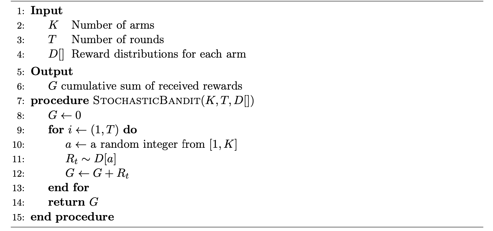
Algorithm 1: Standard stochastic bandit
We see that the stochastic algorithm is quite naïve — it keeps pulling arms at random until it reaches terminal state. This is understandable because the algorithm has no knowledge about the values of the individual actions. It does, however, calculate a cumulative reward \(G\) as
$$ \begin{equation} G = R_1 + R_2 + \dots + R_T = \sum_{t=1}^T R_t \end{equation} $$
Maximising the cumulative reward is one of the central goals of reinforcement learning, as it is underpinned by the reward hypothesis, which states that “the generic objective of maximising reward is enough to drive behaviour that exhibits most if not all abilities that are studied in natural and artificial intelligence” (Silver et al., 2021). What this statement is suggesting, is that the pursuit of a single goal may give rise to complex behaviour and a wide range of abilities, which facilitate the achievement of the goal.
Implementing the K-Armed Bandit Problem in Python
Back to our stochastic bandit. We can write a simple Python implementation that generates synthetic data from a Bernoulli bandit with a specified parameter \(p\)
class BernoulliBandit:

    def __init__(self, p, verbose=True):
        self.p = p
        if verbose:
            print("Creating BernoulliBandit with p = {:.2f}".format(p))

    def pull(self):
        return np.random.binomial(1, self.p)
.Next, we define a BanditsGame class, which runs a simulation using \(K\) bandits with randomly initialised \(p\) values and over \(T\) turns. At each turn, we pull a random arm \(k\) and store the resulting reward as per Algorithm 1.
class BanditsGame:

    def __init__(self, K, T, verbose=True):

        self.T = T
        self.K = K
        self.bandits = [BernoulliBandit(np.random.uniform(), verbose) for i in range(K)]
        self.verbose = verbose

    def run_stochastic(self):

        results = np.zeros((self.T))

        for t in range(self.T):
            k = random.randrange(self.K)
            results[t] = self.bandits[k].pull()
            if self.verbose:
                print("T={} \t Playing bandit {} \t Reward is {:.2f}".format(t, k, results[t]))

        return results
Let's run a simple game featuring 3 bandits over 20 time steps.
game = BanditsGame(K=3, T=20)
game.run_stochastic()
Creating BernoulliBandit with p = 0.21
Creating BernoulliBandit with p = 0.35
Creating BernoulliBandit with p = 0.21
T=0 	 Playing bandit 1 	 Reward is 0.00
T=1 	 Playing bandit 0 	 Reward is 0.00
T=2 	 Playing bandit 1 	 Reward is 1.00
T=3 	 Playing bandit 2 	 Reward is 0.00
T=4 	 Playing bandit 0 	 Reward is 0.00
T=5 	 Playing bandit 2 	 Reward is 0.00
T=6 	 Playing bandit 0 	 Reward is 0.00
T=7 	 Playing bandit 1 	 Reward is 0.00
T=8 	 Playing bandit 1 	 Reward is 0.00
T=9 	 Playing bandit 1 	 Reward is 0.00
T=10 	 Playing bandit 0 	 Reward is 1.00
T=11 	 Playing bandit 1 	 Reward is 1.00
T=12 	 Playing bandit 1 	 Reward is 0.00
T=13 	 Playing bandit 1 	 Reward is 0.00
T=14 	 Playing bandit 1 	 Reward is 0.00
T=15 	 Playing bandit 2 	 Reward is 0.00
T=16 	 Playing bandit 0 	 Reward is 0.00
T=17 	 Playing bandit 1 	 Reward is 1.00
T=18 	 Playing bandit 2 	 Reward is 1.00
T=19 	 Playing bandit 0 	 Reward is 0.00
We observe how the stochastic approach plays a random bandit at each time step, and we also see the corresponding award. Now let's create a function that plays \(N\) number of games, runs each game for a given number of times, and averages the cumulative rewards for each \(n \in N\). The goal here is to use a different set of Bernoulli distributions for each \(n\), but get an idea of the overall performance of each run by averaging the cumulative reward within \(n\). This should give us a good idea about the general performance of the stochastic bandit approach.
def run_simulation(n_runs, runs_per_game, K, T):

    results = np.zeros((K,T))

    for run in range(n_runs):

        run_results = np.zeros((K,T))

        for run in range(runs_per_game):
            game = BanditsGame(K=K, T=T, verbose=False)
            run_results += game.run_stochastic()

        results += run_results / runs_per_game

    results = results / n_runs

    return results
Now let's run the simulation for ten distinct \(\mathcal{D}\)s, 100 runs per set, using 3 bandits and duration of 1,000 turns.
stochastic_results = run_simulation(n_runs=10, runs_per_game=100, K=3, T=1000)
stochastic_results = stochastic_results.mean(axis=0)
print("Mean reward: {:.2f}".format(stochastic_results.mean()))
print("G: {:.2f}".format(stochastic_results.sum()))
Mean reward: 0.49
G: 492.48
We see that the mean reward is very close to 0.5, which is within our expectations. After all, we know that for a Bernoulli random variable \(X\) \(\mathbb{E} [X] = p\). If you look at the constructor of BanditsGame you will notice that \(p\) is sampled from a uniform distribution in \([0,1)\), therefore \(\mathbb{E} [P] = \frac{0+1}{2} = 0.5\).
To get a better picture of the performance of the algorithm, we can also plot the mean rewards achieved by Algorithm 1. Again, we observe, that the mean reward oscillates closely around 0.5.
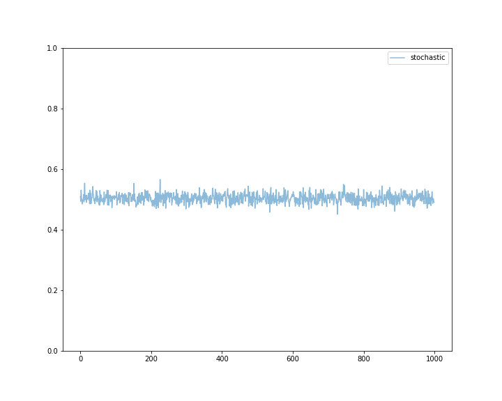
On the other hand, the justification for the value of the cumulative reward doesn’t help with the fact that our algorithm performs similarly to a coin toss. This is not particularly great. However, we'll use this result as a baseline, and in the next blog post in the series, we'll explore several semi-unform strategies that perform significantly better than the baseline.
References
Thompson, W. R. (1933). On the likelihood that one unknown probability exceeds another in view of the evidence of two samples. Biometrika, 25(3-4), 285–294. https://doi.org/10.1093/biomet/25.3-4.285
Silver, D., Singh, S., Precup, D., & Sutton, R. S. (2021). Reward is enough. Artificial Intelligence, 299, 103535. https://doi.org/https://doi.org/10.1016/j.artint.2021.103535

Nikolay Manchev is the Principal Data Scientist for EMEA at Domino Data Lab. In this role, Nikolay helps clients from a wide range of industries tackle challenging machine learning use-cases and successfully integrate predictive analytics in their domain specific workflows. He holds an MSc in Software Technologies, an MSc in Data Science, and is currently undertaking postgraduate research at King's College London. His area of expertise is Machine Learning and Data Science, and his research interests are in neural networks and computational neurobiology.
RELATED TAGS
SHARE

Subscribe to the Domino Newsletter
Receive data science tips and tutorials from leading Data Science leaders, right to your inbox.
By submitting this form you agree to receive communications from Domino related to products and services in accordance with Domino's privacy policy and may opt-out at anytime.