In this post, I discuss a method for A/B testing using Beta-Binomial Hierarchical models to correct for a common pitfall when testing multiple hypotheses. I will compare it to the classical method of using Bernoulli models for p-value, and cover other advantages hierarchical models have over the classical model.
Introduction
Imagine the following scenario: You work for a company that gets most of its online traffic through ads. Your current ads have a 3% click rate, and your boss decides that's not good enough. The marketing team comes up with 26 new ad designs, and as the company's data scientist, it's your job to determine if any of these new ads have a higher click rate than the current ad.
You set up an online experiment where internet users are shown one of the 27 possible ads (the current ad or one of the 26 new designs). After two weeks, you collect the data on each ad: How many users saw it, and how many times it was clicked on.
Time to run some statistical tests! New design A vs current design? No statistically significant difference. New design B vs current design? No statistically significant difference. You keep running tests and continue getting not significant results. Just as you are about to lose hope, new design Z v. current design.... statistically significant difference at the alpha = 0.05 level!
You tell your boss you've found a design that has a higher click rate than the current design, and your company deploys it in production. However, after two months of collecting statistics on the new design, it seems the new design has a click rate of 3%. What went wrong?
When performing A/B testing, data scientists often fall into the common pitfall of failing to correct to for multiple testing. Testing at alpha = 0.05 means your statistical test yielding a result as extreme or more extreme by random chance (assuming a given null hypothesis is true) occurs with probability 0.05. If you run 26 statistical tests, then an upper bound on the expected number of false positives is 26*0.05 = 1.3. This means in our above scenario, our data scientist can expect to have at least one false-positive result, and unfortunately, the false-positive result is the one she reported to her boss.
The Problem
Let's say we are designing Domino's website, and we're testing five different layouts for the landing page. When a user clicks on our site, she sees one of the five landing page layouts. From there, the user can decide whether or not she wants to create an account on Domino.
A | 1055 | 28 | 0.027 | 0.032 |
B | 1057 | 45 | 0.043 | 0.041 |
C | 1065 | 69 | 0.065 | 0.058 |
D | 1039 | 58 | 0.056 | 0.047 |
E | 1046 | 60 | 0.057 | 0.051 |
As a disclaimer, this is simulated data that I created to mimic a real A/B testing data. The number of sign-ups for each website was generated by generating a number from a Binomial distribution with n = Clicks and p = True Rate. The empirical rate represents Sign-ups/Clicks.
Preliminary: Bayesian Statistics
There are two well-known branches of statistics: Frequentist statistics and Bayesian statistics. These two branches have plenty of differences, but we're going to focus on one key difference:
- In frequentist statistics, we assume the parameter(s) of interest are fixed constants. We focus on computing the likelihood Prob(Data | Parameter), the probability we see the observed set of data points given the parameter of interest.
- In Bayesian statistics, we had uncertainty surrounding our parameter(s) of interest, and we mathematically capture our priori uncertainty about these parameters in a prior distribution, formally represented as Prob(Parameter). We focus on computing the posterior distribution Prob(Parameter | Data), representing our posterior uncertainty surrounding the parameter of interest after we have observed data.
Thanks to Bayes's Theorem, we know that the posterior Prob(Parameter | Data) is proportional to Prob(Data | Parameter)·Prob(Parameter), the likelihood multiplied by the prior distribution.
In our problem, the parameters of interest are the true rates at which people sign-up on each website, and the observed data is the number of clicks and sign-ups each website gets. Because we are performing Bayesian statistics, we are interested in modeling the posterior distribution:
Prob(True Sign-Up Rate| Data) ~ Prob(Data|True Sign-Up Rate)·Prob(True Sign-Up Rate).
Classic Bernoulli Model
To build Bayesian models in Python, we'll be using the Bayesian stochastic modeling library PyMC.
import pymcCam Davidson-Pilon has written a great book on Bayesian models in PyMC that I recommend to anyone who is interested in learning Bayesian statistics or how to program Bayesian models in Python. The PyMC code in this section is based on A/B Testing example found in his book.
Before we look at Beta-Binomial Hierarchical model method, let's first look at how we would perform A/B Testing in the standard two website case with Bernoulli models. Recall from above, website A had 1055 clicks and 27 sign-ups, and website B had 1057 clicks and 45 sign-ups.
# Website A had 1055 clicks and 28 sign-ups
values_A = np.hstack(([0]*(1055-28),[1]*28))
# Website B had 1057 clicks and 45 sign-ups
values_B = np.hstack(([0]*(1057-45),[1]*45))
Now, we can model each possible sign-up as a Bernoulli event. Recall the Bernoulli distribution reflects the outcome of a coin flip. With some probability p, the coin flips head, and with probability 1-p, the coin flips tails. The intuition behind this model is as follows: A user visits the website. The user flips a coin. If the coin lands head, the user signs up.
Now, let's say each website has its own coin. Website A has a coin that lands heads with probability pA, and Website B has a coin that lands heads with probability pB. We don't know either probability, but we want to determine if pA < pB or if the reverse is true (There is also the possibility that pA = pB).
Since we have no information or bias about the true values of pA or pB, we will draw these two parameters from a Uniform distribution. In addition, I've created a delta function to create the posterior distribution for the difference of the two distributions.
# Create a uniform prior for the probabilities p_a and p_b
p_A = pymc.Uniform('p_A', 0, 1)
p_B = pymc.Uniform('p_B', 0, 1)
# Creates a posterior distribution of B - A
@pymc.deterministic
def delta(p_A = p_A, p_B = p_B):
    return p_B - p_A
Next, we will create an observation variable for each website that incorporates the sign-up data for each website. We then use pymc to run a MCMC (Markov Chain Monte Carlo) to sample points from each website's posterior distribution. For the uninitiated, MCMC is a class of algorithms for sampling from a desired distribution by constructing an equilibrium distribution that has the properties of the desired distribution. Because the MCMC sampler needs time to converge to the equilibrium, we throw out the first 500,000 sampled points, so we have only points sampled from a (hopefully) converged equilibrium distribution.
# Create the Bernoulli variables for the observation
obs_A = pymc.Bernoulli('obs_A', p_A, value = values_A , observed = True)
obs_B = pymc.Bernoulli('obs_B', p_B, value = values_B , observed = True)
# Create the model and run the sampling
model = pymc.Model([p_A, p_B, delta, values_A, values_B])
mcmc = pymc.MCMC(model)
# Sample 1,000,000 million points and throw out the first 500,000
mcmc.sample(1000000, 500000)
Now, let' examine the posterior of the delta distribution (Remember, this is the posterior of Website B - posterior of Website A).
delta_distribution = mcmc.trace('delta')[:]
sns.kdeplot(delta_distribution, shade = True)
plt.axvline(0.00, color = 'black')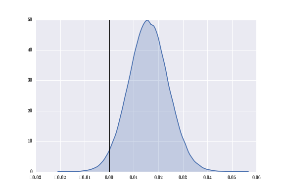
The black line is at x = 0, representing where the difference between the two distributions is 0. From inspection, we see that most of the distribution's mass is to the right of the black line. This means most of the points sampled from B's distribution are larger than those sampled from A's distribution.
To get more quantitative results, we can compute the probability that website A gets more sign-ups than website B.
print("Probability that website A gets MORE sign-ups than site B: %0.3f" % (delta_distribution &lt; 0).mean())
print("Probability that website A gets LESS sign-ups than site B: %0.3f" % (delta_distribution &gt; 0).mean())The probability that website A gets MORE sign-ups than site B: 0.023The probability that website A gets LESS sign-ups than site B: 0.977For these two websites, we see that website B outperforms website A. This worked well for two websites, but if we tried this for all pairs of our five websites, we run the risk of getting a "false positive problem" due to the multiple testing problem. There are 10 possible pairs, so assume we test all possible pairs independently at an alpha = 0.05 level. For each test, we have a 95% chance of not getting a false positive, so the probability that all the tests do not yield a false positive is (0.95)10, which is roughly equal to 0.60. This means the probability of getting at least one false-positive result is about 0.40 or 40%. If we had more websites and thus more pairs to test, the probability of getting a false positive would only increase.
As you can see, without correcting for multiple testing, we run a high risk of encountering a false-positive result. In the next section, I'll show how hierarchical models implicitly correct for this multiple testing pitfall and yield more accurate results.
Beta Distribution
Before I introduce the Beta-Binomial hierarchical model, I want to discuss the theoretical motivation for the Beta distribution. Let's consider the Uniform Distribution over the interval (0,1).

As you can see, it's a simple distribution. It assigns equal probability weight to all points in the domain (0,1), also known as the support of the distribution. However, what if we want a distribution over (0,1) that isn't just flat everywhere?
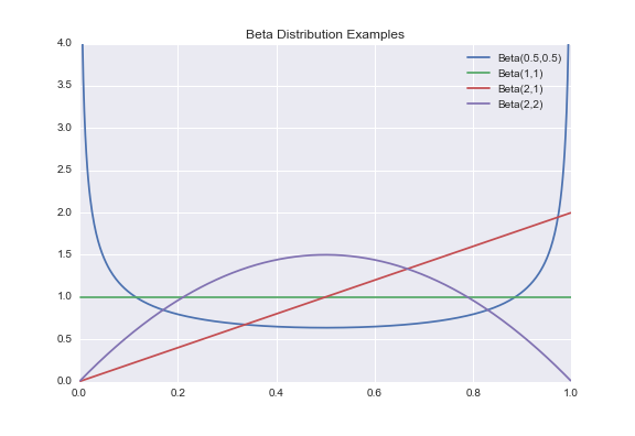
This is where the Beta distribution comes in! The Beta distribution can be seen as a generalization of the Uniform(0,1) as it allows us to define more general probability density functions over the interval (0,1). Using two parameters a and b, the Beta(a,b) distribution is defined with the following probability density function:
Where C is a constant to normalize the integral of the function to 1 (all probability density functions must integrate to 1). This constant is formally known as the Beta Function. By changing the values of a and b, we can change the shape and the "steepness" of the distribution, thus allowing us to easily create a wide variety of functions over the interval (0,1).

Notice in the above plot that the green line corresponding to the distribution Beta(1,1) is the same as that of Uniform(0,1). If you plug in a, b = 1 into the pdf of the Beta distribution, you get pdf(x) = B(1,1)·x1 - 1·(1-x)1-1 = B(1,1)·x0·(1-x)0 = B(1,1)·1·1 = 1, where B(1,1) is the Beta function evaluated at (1,1).
Therefore the pdf of Beta(1,1) is 1 everywhere, so it is equivalent to the pdf of the Uniform(0,1), thus proving that the Beta distribution is indeed a generalization of the Uniform(0,1).
Now, I'm sure many of you are wondering what's the big takeaway from this section, so here they are:
- The Beta Distribution is a versatile family of probability distributions over (0,1).
- This allows us to create prior distributions that incorporate some of our beliefs and thus informative priors.
In the next section, I will discuss why this is important, and how the Beta Distribution can be used for A/B testing.
Hierarchical Modeling
In this section, we will model the website sign-ups using a Binomial Distribution. The intuition behind Binomial(n,p) is that if we flip a coin with probability p of landing heads n times, how likely is it that we see k heads for some k between 0 and n.
In the Classical Bernoulli Method section, I said we had no prior information about the true rates for each website, so we used Uniform(0,1) as our uninformative prior. In this section, we will assume each true sign-ups rate is drawn from a Beta distribution.
Now, the number of sign-ups, ki, is modeled by Binomial(ni,pi), and the true sign-up rate for each website, pi, is drawn from Beta(a,b). Now, we've neglected one important question up until this point? How do we choose a and b?
We could assign a prior distribution to choose these hyper-parameters, but then our prior distribution has a prior distribution and it's priors all the way down.
A better alternative is to sample a and b from the distribution
f(a,b) ~ (a+b)-5/2 where a,b > 0.
I'm sure this function looks like math magic to many of you, but an in-depth explanation of where this probability distribution comes from can be found in Andrew Gelman's book or in this tutorial on Youtube.
The general idea behind this function is that it corporates ideas about the logit of the mean, log(a/b), and the log of the "sample size", log(a+b), to define a proper probability distribution for these two parameters. If the previous sentence means nothing to you, do not worry. All it is saying is that if we use this function, we get desired mathematical properties when sampling for a and b.
Now that I've covered the theory, we can finally build our hierarchical model. The code in this section is based on Stater Stich's Use a Hierarchical Model tutorial.
The beta priors function samples a and b for us from the function defined above. The Stochastic decorator in PyMC requires we return the log-likelihood, so we will be returning the log of (a+b)-2.5.
@pymc.stochastic(dtype=np.float64)
def beta_priors(value=[1.0, 1.0]):
a, b = value
if a &lt;= 0 or b &lt;= 0:
return -np.inf
else:
return np.log(np.power((a + b), -2.5))
a = beta_priors[0]
b = beta_priors[1]We then model the true sign-up rates as Beta distribution and use our observed sign-up data to construct the Binomial distribution. Once again use MCMC to sample 1,000,000 data points from an equilibrium distribution (throwing out the first 500,000 again).
# The hidden, true rate for each website.
true_rates = pymc.Beta('true_rates', a, b, size=5)
# The observed values
trials = np.array([1055, 1057, 1065, 1039, 1046])
successes = np.array([28, 45, 69, 58, 60])
observed_values = pymc.Binomial('observed_values', trials, true_rates, observed=True, value=successes)
model = pymc.Model([a, b, true_rates, observed_values])
mcmc = pymc.MCMC(model)
# Generate 1,000,000 samples, and throw out the first 500,000
mcmc.sample(1000000, 500000)
Let's see what our five posterior distributions look like.
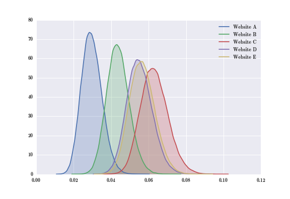
Now that we have all five posterior distributions, we can easily computer the difference between any two of them. In particular, let's look at the difference between Website C and Website A.
diff_CA = mcmc.trace('true_rates')[:][:,2] - mcmc.trace('true_rates')[:][:,0]
sns.kdeplot(diff_CA, shade = True, label = "Difference site C - site A")
plt.axvline(0.0, color = 'black')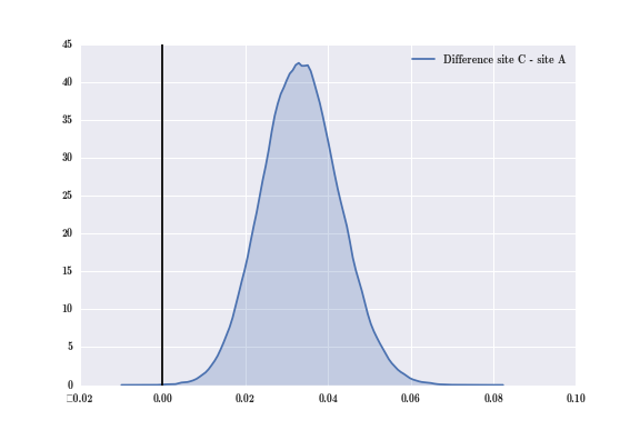
Once again, we see that most of this difference distribution's mass is to the right of the vertical black line, meaning that most of the points sampled from C's distribution are greater than those sampled from A's distribution. If we quantify these results, we get:
print("Probability that website A gets MORE sign-ups than website C: %0.3f" % (diff_CA &lt; 0).mean())
print("Probability that website A gets LESS sign-ups than website C: %0.3f" % (diff_CA &gt; 0).mean())The probability that website A gets MORE sign-ups than website C: 0.000The probability that website A gets LESS sign-ups than website C: 1.000We see that with almost 100% certainty that website C is better than website A. For those of you skeptical of this result, keep in mind that true sign-up rate I chose to simulate data for website C is nearly twice of that of website A, so such a pronounced difference in the posterior distribution of website C and website A is to be expected.
In addition, thanks to the hierarchical model, we can perform multiple tests in succession without having to adjust for multiple comparisons. For example, let's revisit the difference of the posterior distribution of website B and website A.
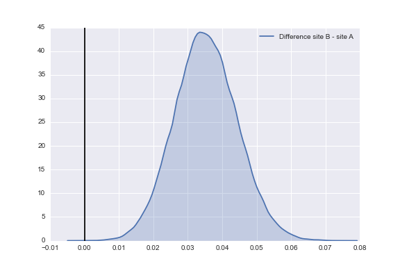
Once again, we see most of the probability mass of this posterior distribution lies to the right of the line x = 0.00. We can quantify these results using the same method we used for the difference between website C and website A.
The probability that website A gets MORE sign-ups than website B: 0.028The probability that website A gets LESS sign-ups than website B: 0.972Again, we see results showing that website B has a higher sign-up rate than website A at a statistically significant level, same as the result when using the classical Bernoulli model.
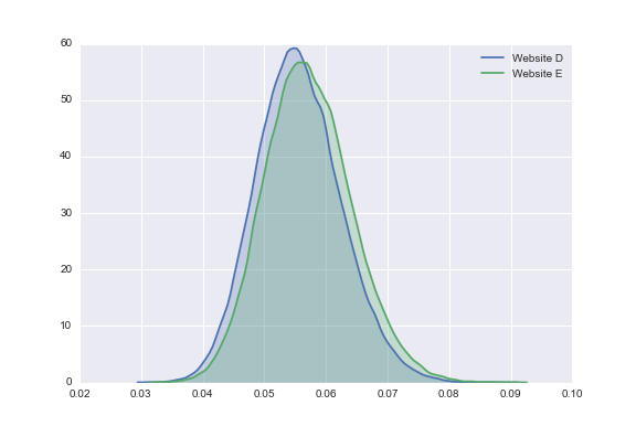
It should be noted that the hierarchical model cannot overcome the limitations of data. For example, let's consider website D and website E. While these two websites have a differing true sign-up rate (website E being better than website D), they have a virtually identical click and sign-up data. If we plot the two posterior distributions for this website, we see they overlap greatly.
As a result, our difference of the posterior yields a distribution centered about 0.0, and we cannot conclude that one website has a higher sign-up rate at a statistically significant level.
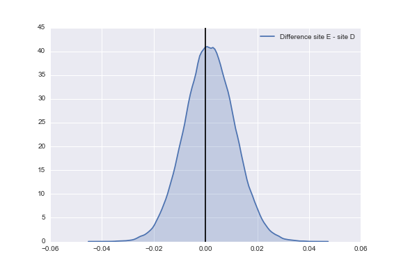
Probability that website D gets MORE sign-ups than website E: 0.437Probability that website D gets LESS sign-ups than website E: 0.563With the hierarchical model, I can test the hypothesis that website C and website A have differing true sign-up rates and the hypothesis that website B and website A have a differing true sign-up rate one after another, something we could not do with the Bernoulli model without making some adjustments to our statistical test.
Comparing the Two Methods
Now I have shown you two different ways to do A/B testing: One way using Bernoulli distributions, and another using Beta-Binomial distributions. I motivated the Beta-Binomial hierarchical model using the problem of multiple comparison testing. Let's now compare the performance of the two methods by examining the posterior distribution generated for Website A by each of the two methods. I've included a black vertical line at x = 0.32, the true rate probability I used to simulate the data.
sns.kdeplot(siteA_distribution, shade = True, label = "Bernoulli Model")
sns.kdeplot(mcmc.trace('true_rates')[:][:,0], shade = True, label = "Hierarchical Beta")
plt.axvline(0.032, color = 'black')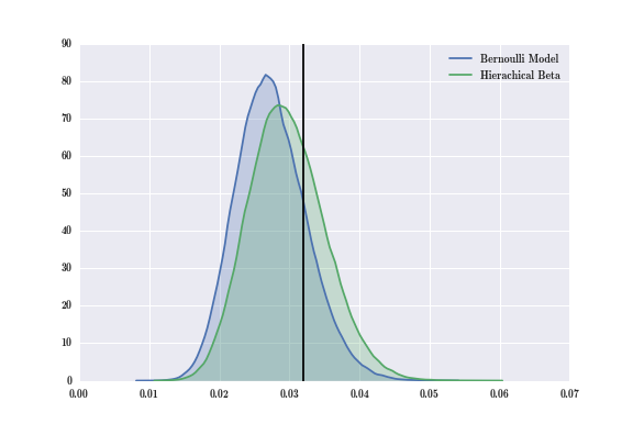
As you can see, the mass of the Hierarchical Beta-Binomial model is closer to the true rate than that of the Bernoulli model. The posteriors of the hierarchical model gave us a closer estimate of the true rate in this case.
Why does the Hierarchical Beta-Binomial model appear to be more accurate in estimating the true rate? Well, this comes down to the prior distributions used in each method. In the classical Bernoulli method, we used the Uniform(0,1) as our prior distribution. As I mentioned earlier, this is an uninformative prior as it assigns equal weight to all possible probabilities. On the other hand, the Beta prior creates a distribution that puts some of the probability mass towards the "truth" and thus we see a more a bit accurate estimate for the posterior distribution. If we slightly altered the values a and b for Beta distribution, it's possible we could see no difference between the two posteriors.
It's possible there is some other mathematical function that we could use as our prior that would result in a more accurate posterior, but we have no guarantees that the resulting posterior would be easily computable. The Beta distribution is a conjugate prior to the Binomial distribution, so we are guaranteed the resulting posterior distribution will be easy to compute (In this case, the posterior will always be a Beta distribution).
Problem of Multiple Testing
Finally, I'm going to address the question everyone has been thinking while reading this! Why do hierarchical models solve the problem of multiple testing?
Let's consider two extremes: In one extreme, we model each website having the same true sign-up rate. This means pA = pB = ... = pE, and thus completely pooling all of the sign-up data from each website together to estimate a "mean" sign-up rate across all five websites. On the other extreme, we model the sign-up rate for each website completely separate from one another and thus focus solely on individual sign-up rates. The Hierarchical models are a compromise between these two extremes, called partial pooling.
In the Hierarchical model, we recognize that since all five websites are modeling the same phenomenon, we ignore some information that holds across all five websites when we model each website in isolation. By incorporating a main effect happening across all five websites while preserving individual effects, we reduce the statistical uncertainty in our models, and thus reducing the issue of multiple comparisons. A more detailed explanation of partial pooling and why Hierarchical models reduce the issue of multiple comparisons can be found in this paper (Section 3.2, pages 7-9).
One important thing to note is that partial pooling is not unique to Bayesian statistics. For example in machine learning, Multi-Task Learning deals with training classifiers to learn a group of related problems using a common representation across all the problems. When we apply a group shrinkage penalty (this mitigates the influence of the common representation on each classifier's decision), we see the partial pooling effect because each classifier's output incorporates the mitigated common representation along with individual representations for each problem.
Lastly, I believe it's worthwhile to mention the most widely known approach to deal with multiple comparisons: The Bonferroni Correction. If you recall from your introductory statistics course, the standard statistical inference procedure revolved around rejected a null hypothesis (H0) if the likelihood of the observed data given the null hypothesis is too small. We quantified what "is too small" meant using an α (alpha) value to represent our threshold for statistical significance (i.e. α = 0.05).
The Bonferroni correction states that if we are going to be testing n hypotheses, then we need to lower our threshold for statistical significance to α/n. For example, if we are planning to test at the α = 0.05 level and we will be testing 10 hypotheses, then the Bonferroni correction states we should test at the 0.05/10 = 0.005 level. This means instead of rejecting our null hypothesis when we get a p-value less than 0.05, we reject our null hypothesis when we observe a p-value of less than 0.005. There are other procedures to correct for multiple comparisons depending on the statistical test involved.
Conclusion
Data scientists use A/B testing to make meaningful impacts on their company's performance. Good A/B testing can lead to million-dollar results, but good A/B testing is also more complicated than you would think. There are many pitfalls that can lead to meaningless results.
Bayesian Hierarchical models provide an easy method for A/B testing that overcomes some of these pitfalls that plague data scientists. This blog post is inspired by Slater Stich's Statistical Advice for A/B Testing series, so anyone interested in learning more about these pitfalls can check out his posts.
If you want further reading on the applied Bayesian method, I recommend this book. In addition to being a good book, it has the most adorable cover. Finally, Udacity recently released a free online course on A/B Testing.

Manojit is a Senior Data Scientist at Microsoft Research where he developed the FairLearn and work to understand data scientist face when applying fairness techniques to their day-to-day work. Previously, Manojit was at JPMorgan Chase on the Global Technology Infrastructure Applied AI team where he worked on explainability for anomaly detection models. Manojit is interested in using my data science skills to solve problems with high societal impact.
SHARE
Other posts you might be interested in


Subscribe to the Domino Newsletter
Receive data science tips and tutorials from leading Data Science leaders, right to your inbox.
By submitting this form you agree to receive communications from Domino related to products and services in accordance with Domino's privacy policy and may opt-out at anytime.