Using Bayesian Methods to Clean Up Human Labels

Session Summary

Derrick Higgins, in a recent Data Science Popup session, delves into how to improve annotation quality using Bayesian methods when collecting and creating a data set. Higgins begins with coverage on models that are part of a “modeling family called probabilistic graphical models”. Probabilistic graphical models are commonly used in Bayesian statistics. Then Higgins walks through “an example based on Gaussian mixture models to demonstrate how you can get started with Stan and build models without too much prior experience in this framework.”

Key highlights from the session include

• Need for labeled or annotated data, with y variables, to do predictions using the supervised model
• Not everyone is given clean data sets, such as the MNIST and Iris data sets used in academia
• Coverage of models such as IRT, MACE, Bayesian Network (Bayes Net), Latent Dirichlet Allocation (LDA), Stan (using PyStan) and more

Higgins wraps up the session by advocating two things: “One is think about your data. Think about how to create data so that it's useful for modeling. Don't just take anything for granted and start modeling right away. And two, graphical models: not as hard as they used to be.”

For more insights from this session, watch the video or read through the transcript.

Video Transcript of Presentation

A lot of the time when you read about data science in the news or in the kind of popular outlets, it can seem like data science is something that starts when you have a data set that you're ready to start working with, that you're satisfied with, and you want to do some modeling. I am going to talk a little bit about the stage that comes before that, where you're actually collecting a data set or creating a data set, and how you can use data science in that process. I'm going to talk a little bit in more detail about what I mean there, and then go into some details about a particular model, using probabilistic graphical models, the background to kind of how that model works, and then present some empirical findings at the end.

When we talk about doing modeling, doing machine learning, most of the time-- say, 90% of the time-- in doing our jobs, we're talking about doing supervised machine learning. So that means we need two things. We need some set of predictors, features, or x variable that we're going to use to parametrize our model. Then we need some set of labeled data, y variables, that we're going use to predict using the supervised model. Where does that come from? Where do we get that? Sometimes it's just given to us. In a lot of academic context or learning contexts, there are data sets that we might just run across or be given; like the Iris dataset; like the MNIST dataset. We don't really have to worry about where they've come from so much.

This a screenshot from Kaggle. If you go there, again, there are a number of data sets that have been curated for us; where we're given a bunch of predictive features; we're given the y variables that go along with them; and all that is asked of data scientists participating in the competition is that they build a model assuming this dataset.

So that's lucky, if you live in that world. You may live in a different world, which is also fairly fortunate, where the thing that you're trying to model is such that there is free data that exists for it. If you want to predict: the rate at which customers will convert, will adopt your platform; you want to predict the rate at which customers will churn and leave your platform; you have some historical data about when that has happened in the past; and you can train your model on that. Or you may have problems that are of a convenient structure, where something like a CAPTCHA will give you exactly the kind of labeled data that you need, and just push your data into this platform. Have users click on these pictures and say which of them include cars or so on. You can use that to train your model.

If you can get free data, again, you know I'd love to live in your world, but typically I don't. More typically-- at least I live in the world-- and I assume this is true of many of you as well, where in order to train a model, you first need to get a set that includes these y variables. That includes these things you're trying to predict and that involves labeling or annotation. There are a number of different types of labeling interfaces or companies that will do labeling for you.

Here's some examples. There's one example up here-- this is-- sorry it's a little too small for you to see. The task here is to look at a picture of a cell cluster and say about how many there are and how they're grouped and so on. This is using information about a wave form of noise to categorize bird calls of different types. This is a text annotation interface; where users might be asked to label particular strings of text: as being particular named entities, as being people or being organizations; so that you can build a model to figure out where people in organizations are in a new text. This is an image annotation interface, where users are asked to draw bounding boxes around particular objects of interest and then label them with that type of object that they are. Then once you've annotated data, like this, you'll have to have a y variable for your model to predict so that it can do object identification.

OK, so that's the setting, where you've got annotation going on. Annotators are imperfect people. They're going to give you some noisy data and you need to figure out how to come up with this-- with reliable data to train your model based on all of these conflicting disagreeing judgments that you get from annotators. And to give you a little background about why I think about the problem the way I do, I'm going to tell you where I've come from.

So right now, I am the manager of the Chicago office of the data science and analytics lab at American Family Insurance. Very much outnumbered by the All State folks so I'm going to ask for a little-- bear with me here. Before I started working American Family, I was at Civis Analytics, here in Chicago. Long time ago, I got my PhD in linguistics back at the University of Chicago. So a lot of the work that I do is natural language processing.

But most of my career I actually spent at the Educational Testing Service, which you may have mixed experiences with. They make the GRE and the TOEFL test, and the SAT and our contract with the College Board. Anyway, they have a lot of texts. They have a lot of essays and interesting data to work on there. So I did NLP there. But I also had the opportunity to work with a lot of psychometricians, who are statisticians who work with testing data or figure out the statistics of how to impute attributes to people based on some observable data.

And one of the major tools that psychometricians use is called Item Response Theory. It's a framework that displaced Classical Test Theory a few decades ago. And this is an example of the kind of equations that are used in Item Response Theory. The idea behind Item Response Theory is that every item on a test is measuring some latent attribute. Something that we want to know about people: it could be about their math ability. If it's a personality test, it could be their openness to new experiences. It could be their psychological stability.

It could be lots of different things you're trying to measure, but every item defines some function that looks like this. It's sort of a sigmoid. And the thing on the x-axis is this attribute. This latent trait. It's a scale. And the thing on the y-axis is the probability that a test taker is going to answer in a certain way, maybe correct, on that test item. The more you know about math, the more likely you are to get the item correct. All the items on a test are you giving you these noisy pieces of information about a student or a test taker; and different test items have different characteristics.

One parameter of this model is the difficulty parameter that moves the curve this way and that way so certain items are harder than others. Another is called the discrimination parameter and that determines how steep this step function is; how well a test item tells a difference between people who don't know the content and people who do. Then there's a guessing parameter as well, which is this floor on the model. So, unfortunately, it's possible to get the answer right if you don't know it. If you just guess. This is a major tool that's used in psychometrics that aggregates all these noisy pieces of information to give you an overall estimate of what somebody knows and can do.

I was really excited, a couple of months ago, when I read about this new paper. Well, actually it wasn't new at the time. It was a couple of years old. It's learning to whom to trust with MACE, where mace stands for Multi Annotator Competence Estimation. It's a model that's really inspired by this IRT, Item Response Theory model, but is used for figuring out-- getting as much information as you can out of annotation. The idea is that, just like each item gives you a noisy piece of information about what a test taker knows, each annotator is giving you a noisy piece of information about the true class that the data they're trying to label should be. I was excited. Even more excited when I found out there was code for this and you can download it.

But it turns out my initial enthusiasm was maybe a little bit misplaced because number one, the download link is broken. That’s a fixable problem. Number two, there's a really, really restrictive license that goes along with the software that means you can't use it for commercial purposes and also from a large set of-- if you're from a large set of countries that I'm sure reflects some defense funding that went into the research behind it. So that was sad. The software couldn't be used for the work that we're doing.

Both this IRT model and the MACE model that I'm going to be talking a little bit about are members of a modeling family called probabilistic graphical models. These models, they're called graphical models because you can draw a graph that represents the dependency relationships between different features or variables in your model. It also includes things like Bayes nets [Bayesian Networks], where you might have a model that's really simple, like this, that says you can observe whether they're sirens going off. You can observe whether there's a traffic jam. And if you know a bunch of-- if you already know whether there's an accident and whether the weather is bad, then knowing that there was a traffic jam doesn't give you any more information about sirens. So that's kind of a model of the way the world works. Not necessarily true, but it's a model that we can make to simplify things and make it more tractable. That's a Bayes Net.

And with more complicated models, like this Latent Dirichlet Allocation [LDA] model, which is a text clustering model that people use a lot, we use a little bit more complicated notation. This is called plate notation, where you specify the dependency relationships between groups of variables. So for LDA, specifically, we have an alpha parameter that determines how concentrated the Dirichlet distribution is for the set of topics in our model. And then we choose a particular categorical distribution, from that Dirichlet distribution, for each document that we have. And then we choose a specific topic from that categorical distribution for each word in the document. And then we generate the words from that topic. So just to say that there is a broad class of these models that fit for different types of problems. I'm going to, in the interest of time, skip past a little bit of the mathematical stuff, but I'm happy to come back it in the question period.

I know a lot of this is second nature for you all, anyway, but-- the models we're going to be talking about are generative models, which means that we're modeling a joint distribution over the x's and y's. Or not making a distinction between the x's and y's here, we could we could set things up differently. These are really useful as in the IRT context when you have labels that are unavailable or only partially observable.

So you don't generally have the ability to know, prior to an examinee taking a test, where they are on the scale. It's something you have to figure out. Yeah. I'm going to skip past the Bayesian terminology here. The posterior is generally what we're interested in. There are a few different ways of coming up with the parameters, in our model, that we want to end up with, where the parameters are something like the annotator reliability estimates or the ability estimates for the students that we're testing. The maximum likelihood estimate is really what we do when we're working in a Non-Bayesian framework. When we don't have any priors that'll just collapse to maximum likelihood. In a Bayesian framework, we want to choose either the MAP, which corresponds to the most likely value of this posterior function that we're trying to estimate or the Bayes estimate, which is the mean over all the possible ways that we can parameterize our model. So those are the metrics.

If you want to actually build a model in this Bayesian framework, historically it's been kind of hard because you'd have to either do some sort of sampling approach -- Monte Carlo approach: Gibbs sampling, or Hamiltonian Monte Carlo, which is both hard to implement and slow. Or you would have to do some ad hoc math for the specific problem you're working on to come up with a variational approximation and then minimize that. There was a high bar to working in this Bayesian framework. However, that's changed in recent years. And there are some toolkits that may make these models much more accessible.

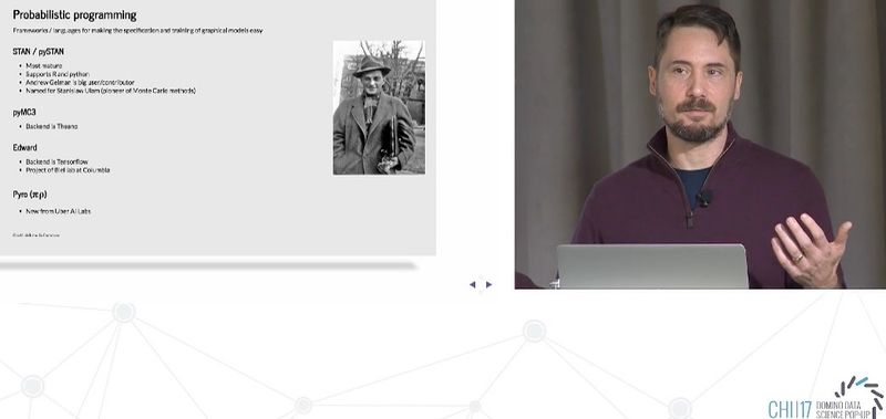
OK. I hope that nothing shorts out. We'll see. The model I'm going to talk about more as this Stan framework, which I'm-- maybe is of more interest because I see there are a lot of R folks in the audience here. It's maybe built out a little bit more fully in R, but there's PyStan as well that allows you to implement these models in Python. And it's not actually an acronym. It's named after this guy Stanislaw Ulam, who was a pioneer of Monte Carlo methods. But there are some other frameworks as well that have been developed in recent years. PyMC3 is on top of Theano, which means it's probably going to go away soon given that Theano is no longer supported. And Edward, which is built on top of TensorFlow. And just in the last couple of weeks, a new toolkit was released by Uber AI, which is called Pyro. I have no experience with that yet, but Stan is pretty mature and it allows you to build these graphical models without worrying too much about the optimization and inference.

I'm going to go through an example based on Gaussian mixture models to demonstrate how you can get started with Stan and build models without too much prior experience in this framework. All you have to do with-- for a Gaussian mixture model is tell it something about your data. First of all, really high level stuff. What's the dimensionality of the data you're trying to model? How many observations do you have? How many Gaussians are you going to try to use in your mixture? And then your data. The actual points are going to fit this mixture of Gaussians to. And then tell it about the parameters of things you're trying to estimate here, phi, from the prior slide. In a Gaussian mixture model there is weight that's associated with each of the Gaussians that determines how they're summed up and then there is a mean that's associated with each of the Gaussians in your mixture. I'm-- to make things simpler, I'm just setting the variance to a constant value. You could change that, certainly. And then, your model doesn't really include anything related to optimization. It's just a specification of what the likelihood is according to your Gaussian mixture model. So you've got a prior. A very weak prior, in this case, on the means of each of your Gaussians. And then to calculate the likelihood, under a given parameterization, you just take all of the points that you've observed and figure out how-- where they fit relative to all the Gaussians and in your mixture. And a little bit of syntax you need to learn about this increment log prob thing here in Stan, but that's, generally, pretty manageable.

OK. So given that, we create some data. Get a function to make some random data that's kind of clumpy. And then we can put it into Stan and tell it to do 1,000 iterations of the no U-turn sampler, which has the built-in general purpose Monte Carlo method for Stan that works well for a lot of problems, and you get output that looks like this. And may or may not be readable, once again, for you. But it's telling you-- OK, there are a bunch of parameters you asked me about and I have computed the Bayes estimate for each of these parameters, given the data that you've input. There are a bunch of thetas for your 10 Gaussians. These are the weights that are associated with each of these Gaussians. And my means are here. There are somewhere between 0.05 and 0.15, maybe. There are the mean values of each of the Gaussians in the x and y plane because we're talking about two dimensional data. And so those are all here. And because we're in a Bayesian framework here, we get a little bit more for free. We're not just getting a point estimate of all these parameters, we're also getting some uncertainties around them so we can see a 50th percentile, which is the median of these parameters across all the samples as well as the extrema. What might be the most extreme values that these parameters are going to take on. And so we can plot this data once you've extracted all these parameter estimates. And hopefully in some of the screens that might be legible, but there are red dots here that indicate the middles of the Gaussians that we fit to this data. And then there is a cloud that, generally, corresponds to the envelope around our data as we would have hoped. So, easy.

All right, back to annotation. This is the idea of the MACE model. The specific model that I was so excited about for trying to get reliable information out of annotators. As with other kinds of Bayesian models, there is a generative story that goes along with this, which means you can tell the conditional dependencies as a narrative about where the data came from. The idea about this labeled data is that you've got end records, that you want to get annotated. Each of those has some underlying category that you don't know, that you're trying to learn. And then you've got M annotators, each of which has some inherent value to them, as a person, which is their reliability, how good an annotator they are; and when one of your M annotators runs up against one of your N data points to be labeled, they flip a weighted coin, and that depends on the reliability value.

If it's over their reliability-- or under their reliability, I guess, they will do the job we've asked them to do and they will get it right 100% of the time. When the coin is tails or wins on the other side, they will just exhibit some random behavior and they will choose a label at random from some distribution, which we're also going to learn. It's not a completely reflective model of the annotation experience that we know because some tasks are harder than others, and when people are trying hard, they can still get the label wrong. But it's, again, good enough for modeling.

If we put this model into Stan, it's a little bit more complicated than the prior one, but not that much. There are a couple more lines here to describe the data. Here we've got I annotated rows, and J annotators, and K annotations, and L annotation categories, and so on. But the meat in the model here, where we're talking about how to calculate the likelihood, is not that much longer. It's only a couple of lines. It didn't take us that much work, which is typically not the case for a lot of these Bayesian graphical models, where there can be a lot of ad hoc adaptation to do.

So how does it work?

There is a data set-- it's a public data set that was used in the original paper and it's Mechanical Turk data. I don't know if any of you've ever used Mechanical Turk for annotation, but it's really, really cheap. You get the quality of annotation that you would expect if you're paying very, very little. So you would expect there to be unreliable annotators in this set and that is, indeed, the case.

For this data set, it was three different actual tasks that annotators completed, and each of these-- each of the rows in each data set was annotated by 10 different turkers. The baseline here is just choose the label that was chosen most frequently by all the turkers that looked at it. So, if there are 10 annotators and six people say one thing and four people said something else, take the mode. The thing that people said six times. And the accuracy, according to that metric, is not bad. Some of these tasks are not very difficult. Like this word sense disambiguation task. We're talking between-- somewhere around 90% to 99%. When your baseline is 99.4%, it's hard to improve on that, and, in fact, using this graphical model does not improve on it. But for some of be other tasks, it does.

So you look at this recognizing textual entailment task. It's a little bit harder. Annotators get-- the mode here-- or the accuracy associated with the mode is 90%. Using this graphical model, you do a little bit better. About 3% better, which is somewhere around a 25% reduction in error. So that's actually substantial. I should say as well, when you're talking about accuracy over here, that's accuracy relative to a trained annotator as opposed to a turker, so there's still some pretty-- there's still some noise in these accuracy estimates. The other thing you can see is your model gives you numbers associated with each annotator that indicate their reliability. These are the underlying thetas or reliability estimates that come out of the model and for different tasks, you get different distributions of this reliability number. But for some of them, you get a very long tail going down all the way to zero. So, basically, some of these people are not trying at all. And beyond using a complicated Bayesian method like this, you might want to consider just excluding these people entirely.

And finally, just to demonstrate the-- that this method isn't only applicable to academic data sets. Here's the same results for an internal data set that's maybe more reflective of the kind of data that people are using in their everyday work. And the characteristics these datasets would have. More categories here. We're talking between 25 and 100 categories as opposed to the two or three categories that annotators are using in the Mechanical Turk tasks. And the number of annotations considerably lower. Between two and five annotations for each task because we're typically not going to get 10 annotations for every row. And even here, you can see there-- you see some spread in the performance of annotators. There are a couple of people down here for some of these tasks who may not be ones that you want to have in your data set that's going to feed into your model training.

These are tools that you can use both to come up with a consensus label, but also for quality control. To make sure that you're managing your annotators. You're looking at their performance in a way that will help you make good decisions about how to annotate data sets in the future.

So, I guess, two things I would hope people take away from this. One, is think about your data. Think about how to create data so that it's useful for modeling. Don't just take anything for granted and start modeling right away. And two, graphical models not as hard as they used to be.

Domino editorial note: this transcript has been lightly edited for readability.