Reproducible Research in Computational Sciences

This guest post was written by Arnu Pretorius, a Masters student in Mathematical Statistics at the MIH Media Lab, Stellenbosch University. Arnu's research interests include machine learning and statistical learning theory.

In science replication is important. The reason is that if the findings of a study can be replicated the stake holders involved in the research are more likely to trust the evidence presented for, or against a proposed hypothesis. Unfortunately, it is not always easy to replicate a study for various reasons. The original study could have been very large (including thousands of participants), expensive or long (stretching over many years). On the other hand, many studies consist of more modest forms of analysis which make them good candidates for replication.

Focusing on the computational sciences, this post looks at how Domino can be used as a tool for reproducible research. The first part will discuss some of the concepts and ideas surrounding reproducible research, with the second part providing a simple example using Domino. Please feel free to skip to any section that is of interest to you.

For a great introduction to reproducible research have a look at Roger Peng's Coursera course, which is part of the Johns Hopkins University Data Science Specialization. In fact, much of the introductory content presented here is based on the slides from the course.

Reproducible Research

Given a scientific article that reports findings from an analysis, the figure below provides three different levels of replication.

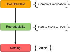
The "Gold Standard" refers to perfect replication. This means that all the necessary resources in terms of the measurement mechanisms, computational hardware and software as well as the steps taken in the analysis are available to such an extent that an exact copy of the original study can be conducted. At the other end of the spectrum is no replication at all. Here only the information regarding the findings provided in the article are given.

Reproducible research lies somewhere in the middle. The idea is to make all the data, code and associated documentation available in such a way that a researcher will be able to reproduce the study. This accessibility is crucial since typically the journey for the reader of an article starts at the opposite end to that of the author (shown below).

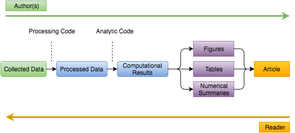
The author moves from left to right, first collecting the data, processing it and then obtaining results through computational analysis. Between each step are code segments that perform tasks to either transform raw data into tidy data or tidy data into results. Finally, all the findings are summarized and condensed into an article consisting of figures, tables and/or numerical summaries. In contrast, the reader who is interested in reproducing the research starts from the right and moves left. Without access to data and code, a reader must decipher what the author did given only the information presented in the article. Therefore, the goal of reproducible research is to essentially give the reader the ability to start from the same position as the author, while at the same time adding the missing pieces between each transformation in the form of code. So, to consider research reproducible by a reader four things are required:

1. The collected data.
2. Processing and analytic code.
3. Data and code documentation.
4. Public access to a distribution platform.

However, difficulties still remain as readers must download data, code and documentation as well as study the documentation to be able to understand which code segment applies to which result and how to rerun the analysis etc. Furthermore, readers might not have access to the same computational resources as was available to the researcher who produced the article. However, the following example shows how Domino can be used to circumvent many of these issues, making reproducing research easier and faster.

An Example using Domino

The data in this example comes from An Introduction to Statistical Learning by Gareth James, Daniela Witten, Trevor Hastie and Robert Tibshirani. It is concerned with studying the relationship between sales of a product and the size of the marketing budget for various mediums such as TV, newspaper and radio.

Note: An outlier was added to the data for the purposes of the example.

Exploratory Data Analysis

Once the raw data has been collected, the first step of an analysis usually involves exploring the data. This is done for TV budgets using the R language.

# read in the dataadsData <- read.csv("Data/Advertising2.csv")# plot sales per thousand from tv advertisinglibrary(ggplot2)ggplot(adsData, aes(x=TV, y=Sales)) + geom_point(col="darkorange") +ylab("Sales (per thousand units)") + xlab("TV budget (per thousand dollars)")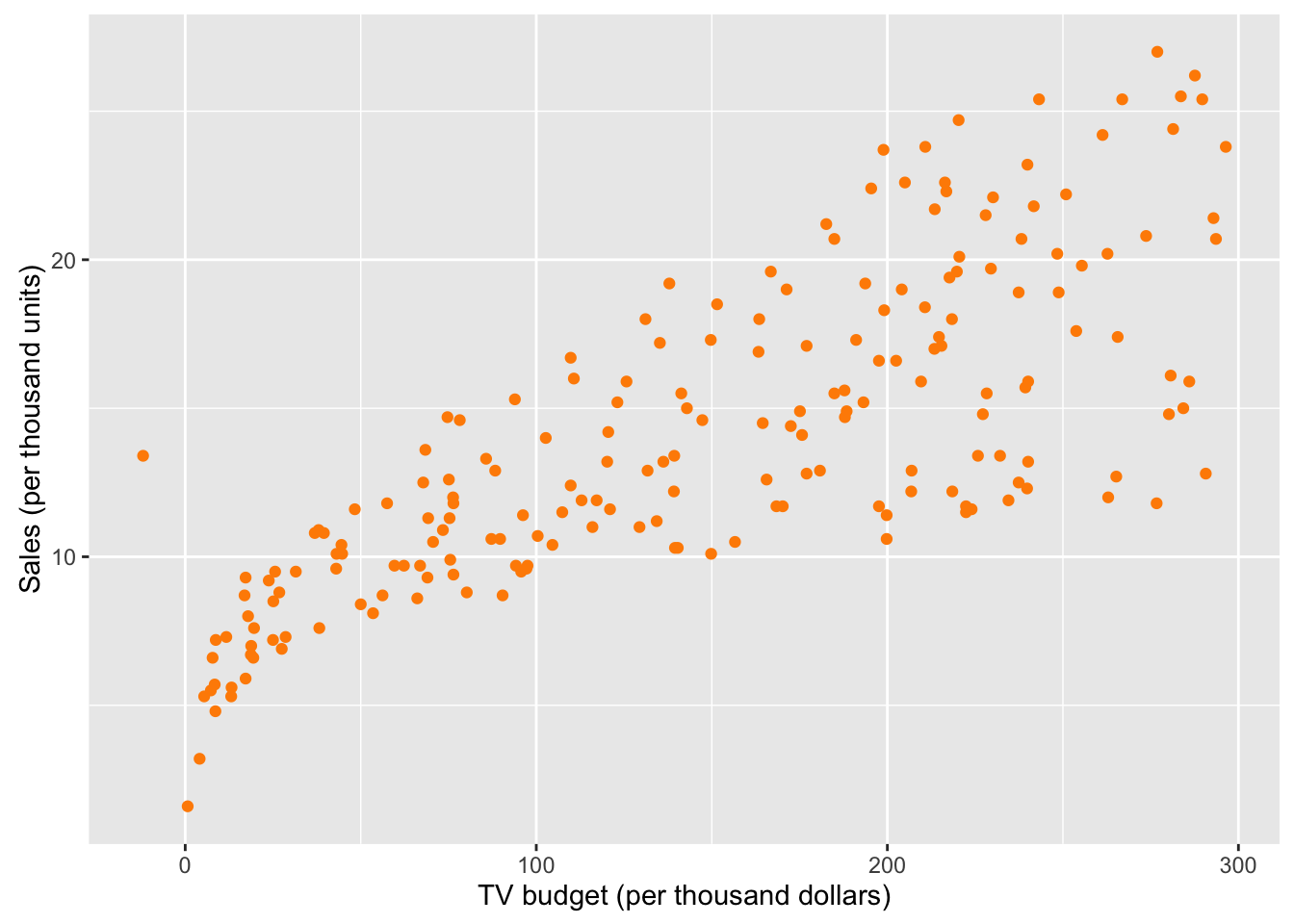

There seems to be a clear positive relationship between the size of a budget and sales. However, a negative budget managed to creep into the data which is most likely a data collection mistake.

Processing Code

The following code removes the point with a negative budget, which resembles the piece of code in the analysis transforming the raw data into processed data.

# processing (remove outlier)outlierIndex <- which(adsData$TV < 0)adsData <- adsData[-outlierIndex,]

Now that the data has been processed the data analytics can be performed.

Analytic Code

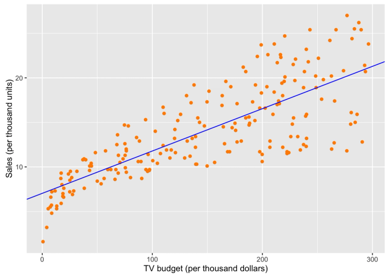
To obtain a more concrete description of the relationship between the budgets and sales, a linear model is fit to the data.

# fit linear model to the datalmFit <- lm(Sales~TV, data=adsData)# print coefficientslmFitCoef <- coef(lmFit)lmFitCoef

## (Intercept) TV## 7.03259355 0.04753664

According to the linear fit increasing the TV budget by a thousand dollars will roughly result in an extra 47 units sold. The fit is plotted below.

# plot fitggplot(adsData, aes(x=TV, y=Sales)) + geom_point(col="darkorange") +geom_abline(intercept = lmFitCoef[1], slope = lmFitCoef[2], col="blue") +ylab("Sales (per thousand units)") + xlab("TV budget (per thousand dollars)")

Now that the analysis is complete, let's see how Domino can be used to reproduce the results.

Reproducibility using Domino

In a nutshell, Domino is an enterprise-grade platform that enables data scientists to run, scale, share, and deploy analytical models. This post by Jo-Fai Chow includes a tutorial on how to get started with Domino, from getting up and running, to running your first analysis in the cloud. Alternatively, you can sign up for a live demo to see what Domino has to offer. So let us get started.

The code below represents the full analysis pipeline that was created to perform all the necessary steps to transform the raw advertising data into a computational result in the form of a linear fit. The code was saved as lmFitAdvertising.R.

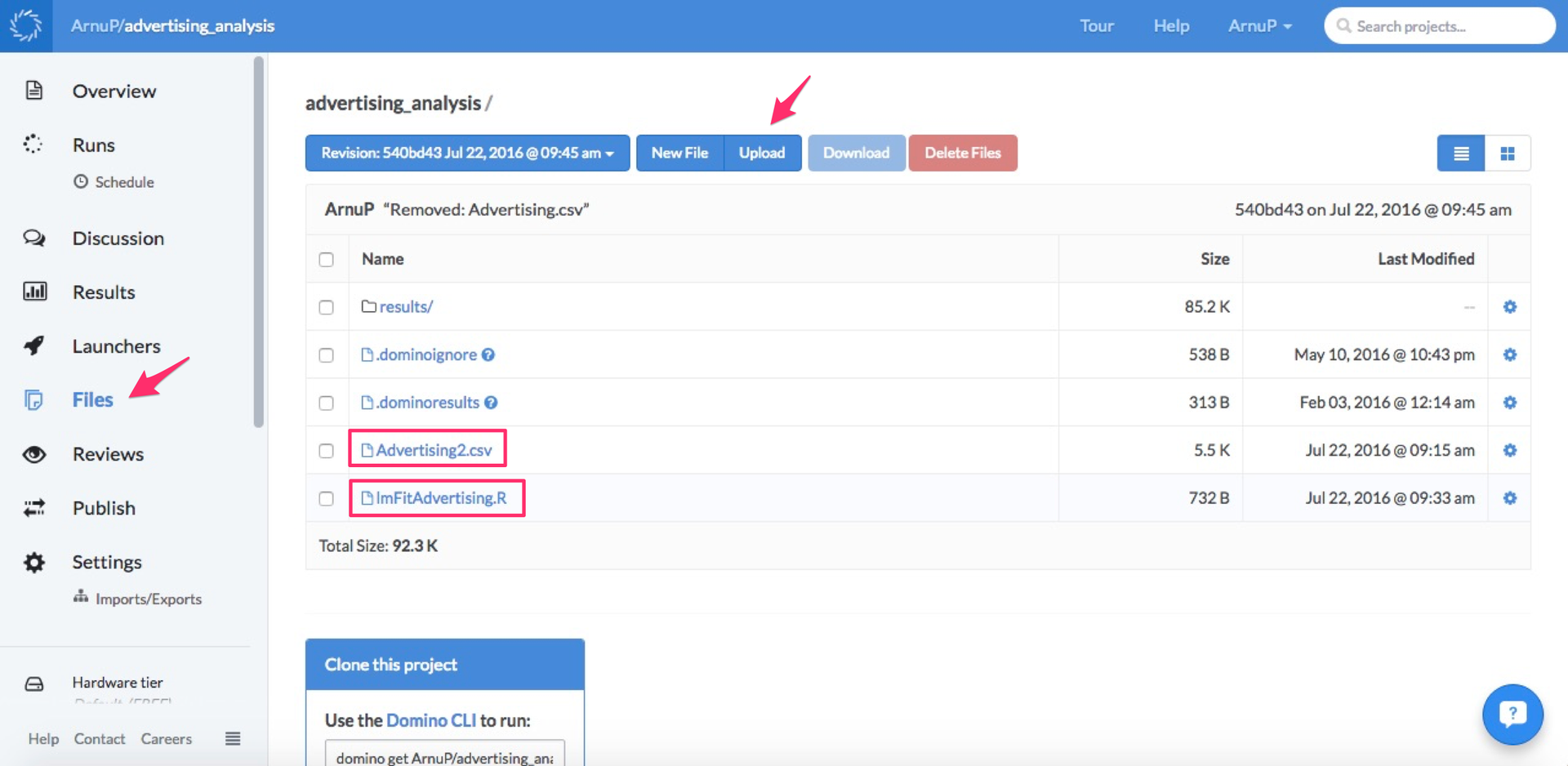
########################################################## Fit linear regression model to the advertising data ########################################################### read in the dataadsData<- read.csv("Advertising2.csv")# processing (remove outlier)outlierIndex <- which(adsData$TV < 0)adsData <- adsData[-outlierIndex,]# fit linear model to the datalmFit <- lm(Sales~TV, data=adsData)# print coefficientslmFitCoef <- coef(lmFit)lmFitCoef# plot linear fitlibrary(ggplot2)ggplot(adsData, aes(x=TV, y=Sales)) + geom_point(col="darkorange") +geom_abline(intercept = lmFitCoef[1], slope = lmFitCoef[2], col="blue") +ylab("Sales (per thousand units)") + xlab("TV budget (per thousand dollars)")

The first step in making the analysis reproducible is to ensure that all the required data and code are located within the Domino project files. If the entire analysis was performed using Domino the files should already exist inside the project, but Domino also allows for data and code to be uploaded as shown below.

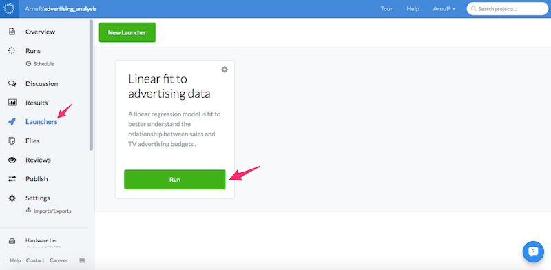
Next navigate to the Launchers page to create a new Launcher. These are self-service web forms that run on top of the analysis code.

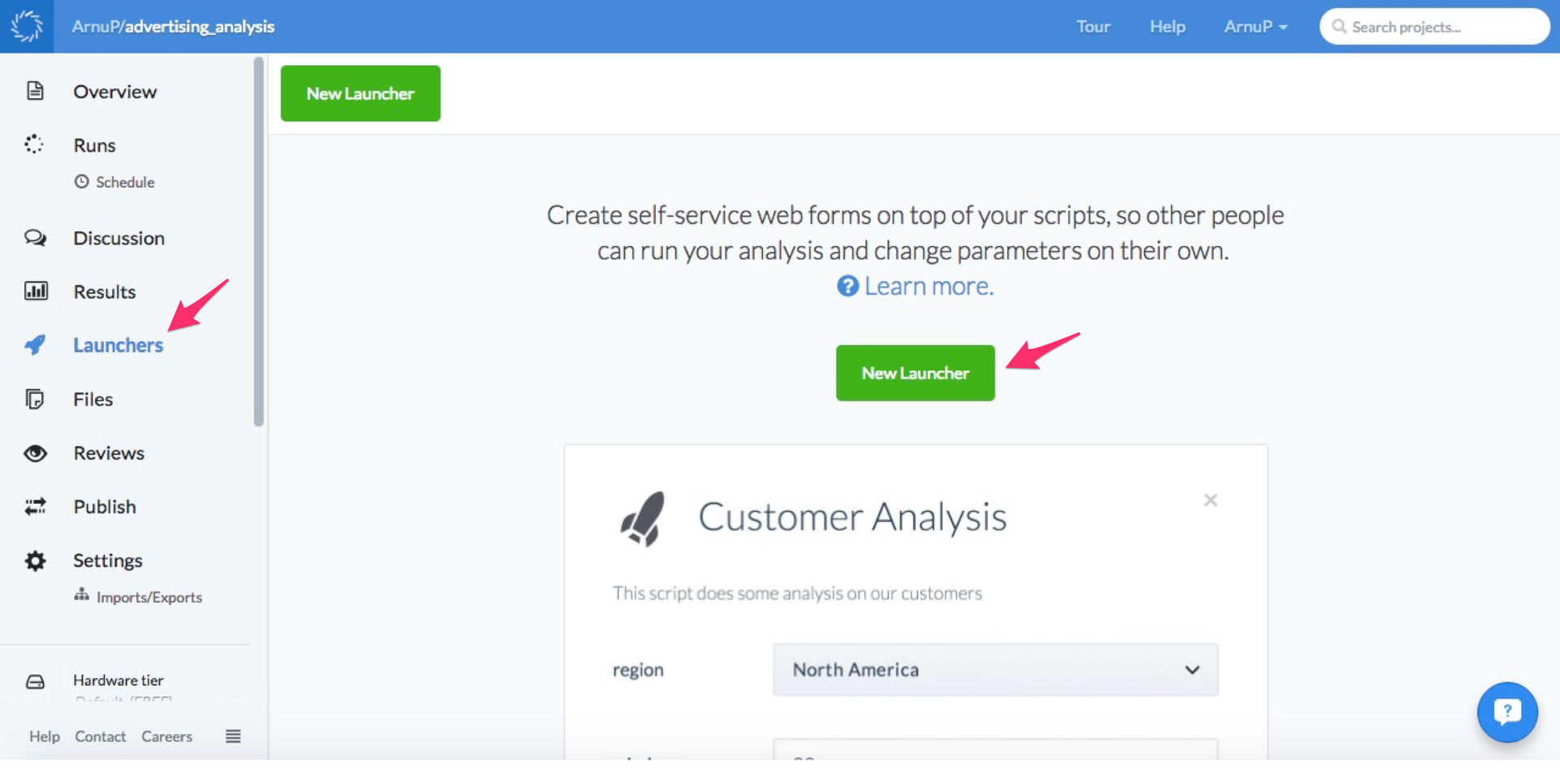
To create a launcher simply click on the New Launcher button, give it a name and a description and select which program the launcher should run (in this case lmFitAdvertising.R).

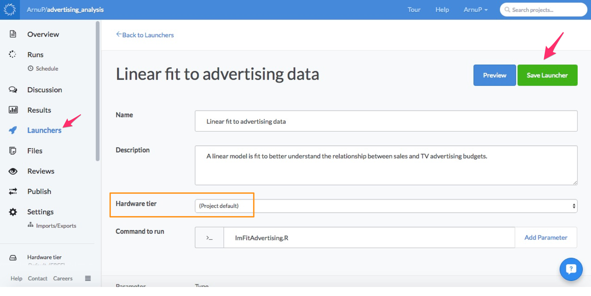
One more available option is to set the Hardware tier, which is set to "project default" in this example. This option is really useful. If all the analysis was originally conducted using Domino, the researcher can remove possible computational barriers for the reader by ensuring that the same hardware tier used in the analysis, is also selected for the launcher. Finally, save the launcher by clicking on Save Launcher in the top right.

Before the launcher can be accessed publicly the project settings must be changed. Head over to Settings and click on the Access & Sharing tab.

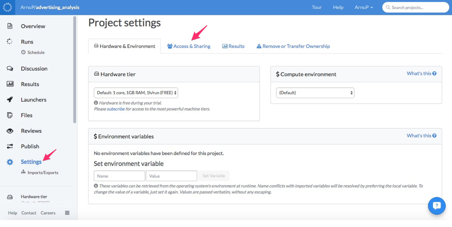
Inside Access & Sharing select the Public: Viewable by anyone options and tick the Allow run execution by anonymous users box.

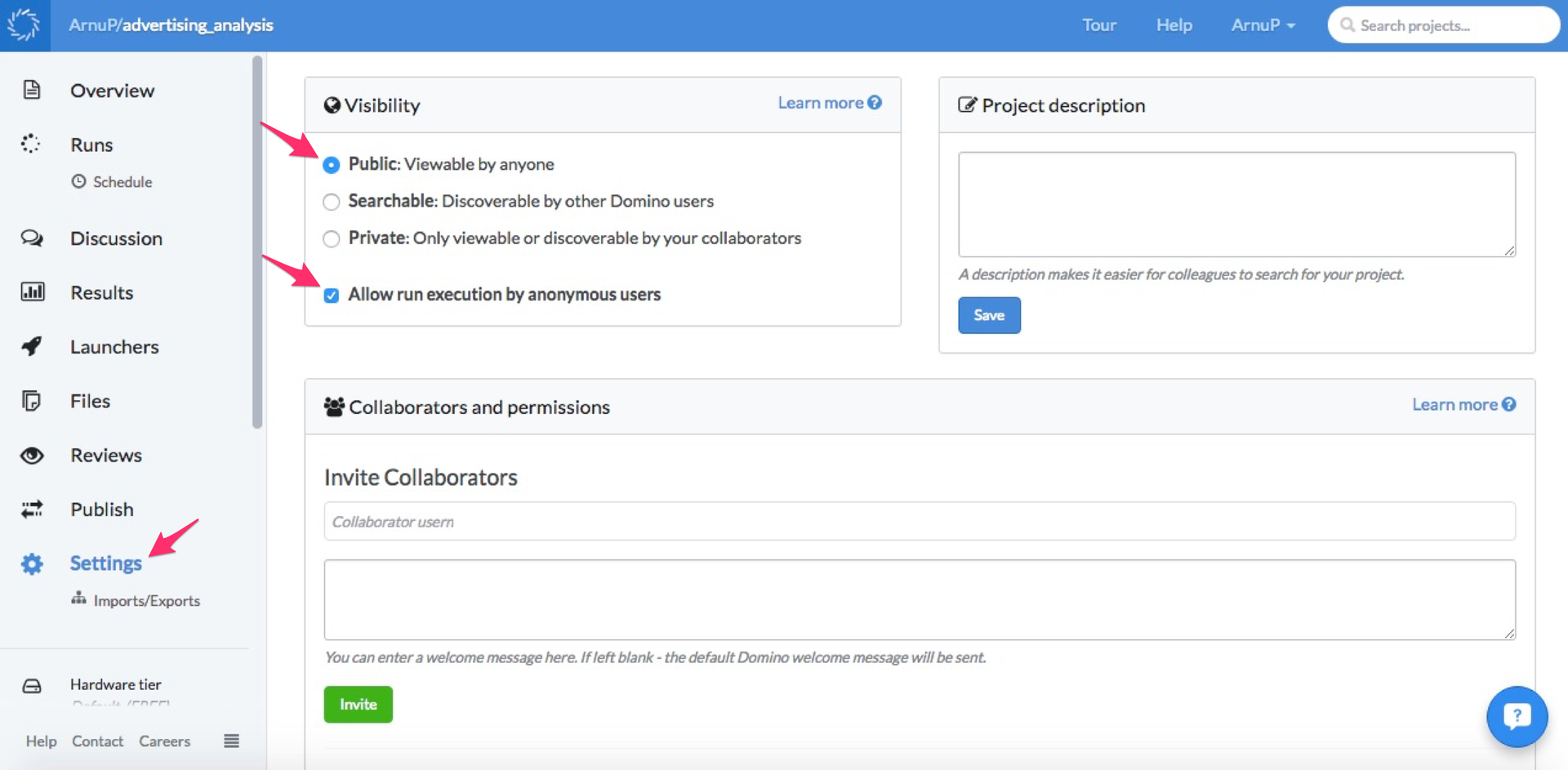
These settings will make the project publicly accessible and will allow anyone with a URL pointing to the Launchers page to run a launcher. So everything is now setup on Domino's side.

This example will use LaTeX but the steps are likely very similar for Word. The code below shows a table (as might typical appear in an article) presenting the results of the linear fit (the regression coefficients).

\documentclass{article}\usepackage{hyperref}\begin{document}\begin{table}[!htbp] \centering\caption{Linear fit to advertising data}\href{https://trial.dominodatalab.com/u/ArnuP/advertising_analysis/runLaunchers}{\begin{tabular}{@{\extracolsep{5pt}} cc}%\\[-1.8ex]\hline\hline \\[-1.8ex]\textbf{Intercept} & \textbf{TV (Slope)} \\\hline \\[-1.8ex]$7.0326$ & $0.0475$ \\\hline \\[-1.8ex]\end{tabular}}\end{table}\end{document}

By wrapping the tabular in an href tag using the hyperref package, the table can be made clickable, linking to any given address on the web. Therefore, by inserting the Launchers page URL, a reader with an electronic version of the article will be able to click on the table and be directed to the launcher fitting the linear model. The results can be reproduced by clicking on the Run button.

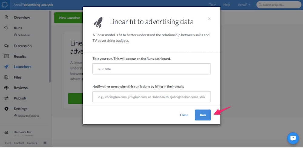
Domino provides the option to change the title of the run as well as send the results to a specified email address. Once these are filled in (or left blank) the reader clicks Run again.

The code printouts are displayed as the code is run. The coefficients can be viewed in the red box below.

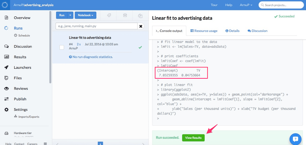
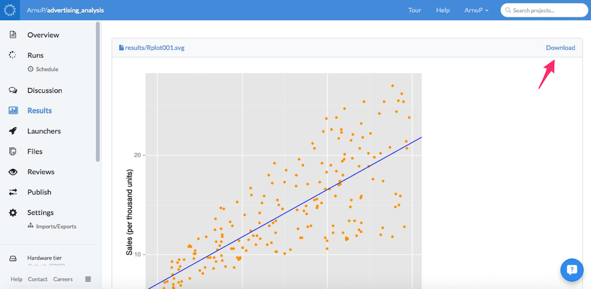
To view the plot the reader can click on View Results. Here, both the coefficients and the plot will be displayed. The plot can then be downloaded using the button situated at top right corner.

So there it is, reproducible research using Domino. In summary, Domino allows the author to:

• Do the entire analysis in the cloud.
• Download the computational results to be used in an article.
• Make the results reproducible by creating publicly accessible launchers and linking them to the electronic version of their article.

The reader is then relieved of the following tasks:

• Downloading the data, code and documentation required to reproduce the findings.
• Assuring that adequate computational power is available to rerun the analysis.

A working version of the example can be found here. It includes the built LaTeX files with the produced PDF containing the table presented earlier. The PDF will direct you to the launcher reproducing the example. You can also access the Launcher directly by visiting the project on the Domino platform.