R in Ecology

I’m a bit of an R nerd. Ok, that’s a lie; I’m a major R nerd. But for good reason, because R is incredibly useful in streamlining the scientific process, and increasing the ability to replicate findings with less human error.

The main reason that I often talk to my fellow graduate students about learning R is because of the near constant that a graduate student has to redo things; this even happens within science as a whole. If you spend an entire week using a GUI to run all of your models, then you present them to your advisor, and s/he tells you that you need to change “just one thing,” it will take you another week to do so. This is frustrating, to say the least, especially when it happens more than once.

However, when you have scripted that process, it is often much faster and easier to go back and make small changes without having to redo large parts of your work by hand, or remember every step of the process. This is true whether you are summarizing your data, running models, or making graphs. The learning curve is steep, but particularly if you plan to continue to conduct research after you receive your degree, it is very much worth it. It is also helpful when you are working on multiple projects and you might not touch the data for three months, and then need to jump right back in. If you have described your scripts well (you have a file with the code and lots of detail about what is going on) you can resume the project more easily, remember where you left off, why you dropped all the data from site 23, and what kind of model you ran. Right now, I’m juggling five dissertation chapters and three side projects. My to-do list and R scripts are the only things that allow me to keep my head above water.

In addition, it is helpful when you need to add more data to your analysis, either because more have been collected or because you analyzed only a subset of the data before. Noam Ross has some nice slides that describe why replicable research is a valuable goal. These slides discuss some other tools, but the concepts apply very well to R. R can help you make your analysis as transparent as possible, and eliminate the need to rerun the it constantly, and regenerate graphs that incorporate that pesky “one more fix.”

Data Cleaning

I don’t enter my data in R. Some do, but I find it tedious, and also have my technician enter about half of my data, as it is easier to use a spreadsheet. Once it has been entered and proofed, however, I export it to .csv, and script everything else in R. I have an awful memory. I never remember what I did with my data, so I script it so I can look back and figure everything out and redo it if/WHEN I need to. I NEVER change the raw data file (the original one that was entered from my field data sheets). Any alterations of that data are done within R and then written to a different .csv.

The first part of the process is data cleaning. As much as I talk about #otherpeoplesdata on Twitter, I often spend a great deal of time cleaning my own data. This involves checking for numeric values that are impossible, and often for misspellings. Because I collect my data over a three-month period each fall, it also lets me explore the data along the way and see what is going on.

Cleaning data may sound tedious, and it can be, but it is very important. Otherwise when you try to run an analysis or summarize your data and get summaries of water depth for “missouri,” “Missouri,” and “MiSsouri,” it is less than helpful.

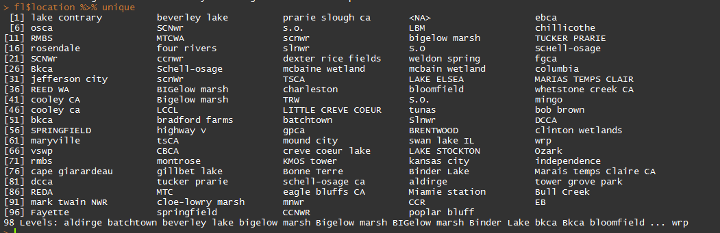
Here is an example of all of the unique location values for a different dataset with which I’ve been working. As you can see, there are many inconsistencies: Bigelow marsh and BIGelow marsh, for instance.

In addition, if you have a dataset that will grow over time, you can use this method to combine data files from all those different periods in one script, so that you don’t have to paste, copy, and worry about destroying anything. This is also very helpful if you are receiving data from different people, so you can make sure it’s all in the same format.

This method also retains the original files, as they are in case you need to go back later and figure out the source of any strange values. Each morning during my fieldwork, I export the survey data from our GPS management software and clean them/check them/stitch them together using the “combining_night_files.R.”

file_names <- list.files (path=”./R_in_ecology/night_files/“,pattern=“.csv”) 
# creates a list of the files so that we can read all of them in, and not have to copy and paste all the file names, or worry about updating that list manually as the files grow in number. These data are highly subsetted files from my dissertation, and I realize that latitude typically is accompanied by longitude, but this is all I’m using for this example.  

library(tidyr)
library(dplyr) # gives us the gift of pipes “%>%” 
library(auriel) # my personal R package, used here for the ordinal_date_con() function
nights <- list() # creates the list into which all of our files are going to be stored
for(i in 1:length(file_names)){
# first I have to pull the data I need out of the file name, as I store a bunch of information there.
  dat <- as.data.frame(file_names[i]) 
  colnames(dat) <- “name”
  names <- dat %>% separate(name, into=c(“year”,”month”,”day”,”obs”,”round”,”region”,”area”,”impound”,”treat”,”night”),sep=“_”)
  names <- names %>% separate(night, into=c(“night”,”file”), sep=-5)
 # now we read in the .csv and stitch together all of the data from above with this data   frame, as well as splitting things apart into multiple columns
  int <-  read.csv(paste0(“./R_in_ecology/night_files/“,file_names[i]))
  lesscol <-  int[,c(“lat”,“name”)]
  lesscol$name <- as.character(lesscol$name)
  lesscol$name <-  ifelse(nchar(lesscol$name)==7,paste0(lesscol$name, “N”),lesscol$name)
  lesscol <- lesscol %>% separate(name, into=c(“name”,“distance”),sep=5) %>%  separate(distance, into=c(“species”,“distance”), sep=1) %>% separate(distance, into=c
  (“distance”,“flush_walk”), sep=-2)
  lesscol$distance <- as.numeric(lesscol$distance)
  lesscol$species <- tolower(lesscol$species)
  lesscol$year <- as.numeric(names$year)
  lesscol$month <- as.numeric(names$month)
  lesscol$day <- as.numeric(names$day)
  lesscol$obs <- names$obs
  lesscol$round <- names$round
  lesscol$region <- names$region
  lesscol$area <- names$area
  lesscol$impound <- names$impound
  lesscol$treat <- names$treat
  lesscol$night <- names$night
  lesscol$odat <- ordinal_date_con(lesscol[,c(“month”,“day”,“year”)])
  nights[[i]] <- lesscol # throws it back into the list in the same place it came from; some will hate this.
  }
  masterdat <- do.call(rbind, nights) #: this binds together all of the items in the nights[[]] list. This script is great because it can grow with each file.
 # now we can write this out, or do whatever needs to be done with it. 

I also have a script for our survey and vegetation data. Same process, loop through, and check each file individually, check it over, and then stitch them together. The example data files on github have one file for the sake of simplicity.

I use amazing things like match (%in%) to make sure my plants are spelled correctly and my sites don’t have typos, so that later when I start to analyze my data, I don’t have to spend a lot of time proofing it.

int <- read.csv(“./R_in_ecology/example_survey_data.csv”)
regions <- c(“nw”,“nc”,“ne”,“se”)
fs <- c(“fed”,“stat”)
print(paste0(int[(int$region %in% regions==FALSE),]$region,“ ”, “region”))
print(paste0(int[(int$fs %in% fs==FALSE),]$area,“ ”,“area”))
is.numeric(dat$sora)
is.numeric(dat$jdate)

When this file just returns a bunch of “region” and “area” instead of “SDF region” or whatever other incorrect value is there, we are good to go. When I do this over the 100+ files I collect throughout the season, I will run it with a “for” loop to check each one individually.

The dplyr and tidyr packages are essential in making all of this happen.

Reports

One of the main ways that I use R almost every day is through RMarkdown files, which allow me to eliminate some of the pain-in-the-butt-ness in writing reports and regenerating a series of graphs. I can write it in R and knit it all together, and come out with a nice looking and clear .html or .pdf file.

This is SUPER GREAT for creating regular reports for collaborators, or for generating a bunch of graphs every day without having to do a bunch of work (work smart, not hard!).

It takes all of the copy and paste out of the process, and can make BEAUTIFUL REPORTS with ease. I love RMarkdown; it is simply the best. Now if only I could get all of my collaborators to write in it as well. Instead, I send them .pdfs, and they give me comments, which also works. This is a good place to start with RMarkdown.

What is great is you can write things like this:

# Fun with GraphsYou can create graphs in RMarkdown and print them with or without the code shown. The echo, message, and warning arguments are set to false in the first graph to hide the code and any other outputs.{r, echo=F, message=F, warning=F}dat <- read.csv(‘./example_survey_data.csv’)gdat <- dat[,c(“jdate”,“sora”)] %>%group_by(jdate) %>% summarise_each(funs(median))ggplot(data=gdat) +geom_bar(aes(x=jdate, y=sora), stat=“identity”)+theme_krementz()+scale_x_ordinaldate(year=2015)+xlab(“date”)+ylab(“sora per hectare”)

and knit it and get this.

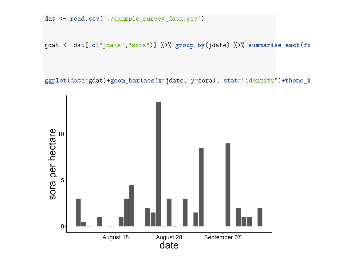
Pretty cool, eh? Not having to export graphs, copy and paste them into Word, and deal with formatting and such is a huge lifesaver, and can make it much easier to create reports regularly with the same graphs/tables and other data analyses. I use this for my regular fieldwork reports, for my annual report that contains over 50 maps and 25 figures, and for many other smaller products that I use daily/weekly/monthly. You can also include latex code in the markdown document to help customize it more. I do this for my CV.

Graphing

I adore ggplot2. I get a ridiculous amount of joy out of making a huge number of beautiful graphs. Tweaking graphs is what I do when I’m frustrated with the rest of my dissertation.

ggplot is a great way to make publication quality graphs that can be used for presentations, or to make fun graphics, and they are generated through those RMarkdown reports that I mentioned earlier that I use to keep an eye on my data and create updates for collaborators.

One of the things I love about ggplot is that I have built a custom theme named for my adviser that makes graphs that he likes, which saves me A TON of time, which is a valuable thing, and helps keep my adviser happy, which is an even more valuable thing. Therefore, instead of having to write out/copy and paste this every time I want to make a graph that looks the way I want:

ggplot(data=masterdat)+
   geom_histogram(aes(x=odat))+
   scale_x_ordinaldate(2015)+
   theme(axis.text.x = element_text(size=12,color=“black”),
     axis.text.y = element_text(size=12,color=“black”),
     axis.title.y=element_text(size=20),
     plot.background = element_blank(),
     panel.border=element_blank(),
     panel.grid.major= element_line(colour=NA), 
     panel.grid.minor=element_line(colour=NA),
     title=element_text(size=20),
     panel.background = element_rect(fill =“white”),
     axis.line=element_line(colour=“black”),
     strip.background=element_rect(fill=“white”, color=“black”),
     strip.text=element_text(size=15))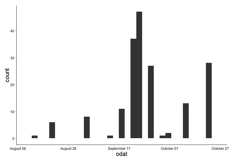

I can write this:

ggplot(data=masterdat) +   geom_histogram(aes(x=odat)) +   scale_x_ordinaldate(2015) +   theme_krementz()

This is shorter, cleaner, and doesn’t require me to remember a whole lot, which is honestly my goal in every R script, to save my poor memory.

Custom R Packages

Having your own R package is really useful; it’s a great place to save things like custom themes for ggplot, and also useful mods for other parts of ggplot, like this one.

I keep all of my dates in ordinal date (day of the year) and so I built this custom scaler for ggplot that makes it a snap to create graphs that have real looking dates (August 1), instead of ordinal dates.

scale_x_ordinaldate <- function(year){   scale_x_continuous(label=function(x) strftime(chron(x, origin=c(month=1, day=1,year=year)), “%B %d”))}

So I can just add scale_x_ordinaldate(2015) onto my ggplot graph and it will change my ordinal dates (day of the year) in my graph to more readable dates (August 1).

Hilary Parker has written a great intro on creating your own R package. This is perfect for saving and using functions you have written, and for saving datasets that you need to see frequently. I use the same datasets in many, many projects, and if I just worked on one computer, this wouldn’t be a big deal. I could use file paths to keep everything organized and saved in one folder somewhere. Instead, however, in an average week, I work on two, if not three, different computers, so these file paths just cause frustration, if they don’t waste a ton of my time.

There are a few ways to circumvent this, but one of them that Oliver Keyes and Jeff Hollister suggested to me was to save those data files into an R package. Then you just load the package onto your computer and bam, data files. These data files can be updated easily, and by using github, you can move the packages between computers easily. You don’t have to worry about any issues of data privacy, as you can have private packages. On github, though, if you don’t have the education discount, you will have to pay for them (bitbucket is one way of getting around this).

Saving data in an R package also helps encourage you (though it does not force you) to document your data, which is often one of the big issues when you hand your data over to someone else—lack of documentation (what do all of those column headers mean anyway?).

This is also great practice for writing and troubleshooting functions, and maintaining a package so someday you can work on packages that you will share with others. Maybe you’ll never do that, but knowing how packages work, and how to troubleshoot them can save you a ton of headaches in the future.

You can check out some functions I often use with my personal R package here. I’ve got a private data package as well, but sadly, I cannot share it publicly.

Modeling

Most of the modeling I do, and most of the headaches in my day are all because of package “unmarked,” which allows me to use distance sampling data to examine questions about the density of birds within habitats and study their migration.

There are so many ways to model in R, and so many different kinds. I’m most familiar with the hierarchical models supported by unmarked. These models allow estimation of the abundance of animals, occupancy (or availability) and detection probability at the same time, which is very powerful, and allows me to use a variety of covariates to explain each level of the model.

How to get started with R

One reason I really like using R is how flexible it can be in making the re-arrangement of data straightforward so that when my collaborators come back with yet another new way of thinking about the data, I can rearrange things quickly and carry on running the models. It helps remove a lot of the memory from conducting science, which is a good thing, and it also allows you to go back and figure out where things went wrong when they do (because they will).

R does have a learning curve, especially if you’ve never programmed before, but it can be very fun and rewarding, and once you are over the learning curve it's super powerful.

I’m an instructor for Software Carpentry and Data Carpentry, and their lessons, which are available on their websites, are fantastic. I often direct people to start with Software Carpentry to get a handle on the R language before diving into Data Carpentry, but it really depends where you and what your goals are.

Packages like tidyr and dplyr are great for cleaning, organizing, and manipulating your data within a set of consistent functions. Both were written by Hadley Wickham who is an active member of the R community, with which I recommend people get involved via Twitter.

The #rstats hashtag on Twitter is a great place to go and ask questions, and I often receive multiple helpful responses within 20 minutes. Moreover, it’s a good place to escape from the snark that can plague other sources of R help.