Performing Non-Compartmental Analysis with Julia and Pumas AI

When analysing pharmacokinetic data to determine the degree of exposure of a drug and associated pharmacokinetic parameters (e.g., clearance, elimination half-life, maximum observed concentration $$C_{max}$$, time when the maximum concentration was observed $$T_{max}$$, Non-Compartmental Analysis (NCA) is usually the preferred approach [1].

What is Non-Compartmental Analysis (NCA)?

At its core, NCA is based on applying the trapezoidal rule from numerical analysis against the plasma concentration-time curve to calculate the area under the curve (AUC) and the area under the first moment curve (AUMC). To calculate the area under the curve for a given time interval, say from [latex]t_0[/latex] to time of last blood sample [latex]t_{last}[/latex], we need to solve the following integral of the rate of change of concentration in plasma as a function of time.

$$

{AUC}=\int_{t_0}^{t_{last}}C(t)dt
$$

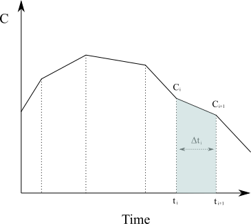
Approximating the region under the graph of [latex]C(t)[/latex] as a series of trapezoids and calculating the sum of their area (in the case of [latex]N[/latex] non-uniformly distributed data points) is given by

$$

{AUC}=\int_{t_0}^{t_{last}}C(t)dt \approx \sum_{i=1}^{N}\frac{C(t_{i-1})+C(t_i)}{2}\Delta t_{i}
$$

The area under the first moment curve would respectively be

$$

{AUMC}=\int_{t_0}^{t_{last}} t \times C(t)dt \approx \sum_{i=1}^{N} \frac{t_{i-1} \times C(t_{i-1})+t_i \times C(t_i)}{2} \Delta t_i
$$

Having calculated AUC/AUMC, we can further derive a number of useful metrics like:

• Total clearance of the drug from plasma $$CL=\frac{Dose}{AUC}$$
• Mean residence time $$MRT=\frac{\text{AUMC}}{\text{AUC}}$$
• Terminal disposition rate constant $$\lambda z=\frac{\text{CL}}{\text{volume of distribution}}$$

NCA doesn't require the assumption of a specific compartmental model for either drug or metabolite; it is instead assumption-free and therefore easily automated [1].

PharmaceUtical Modeling And Simulation (or PUMAS) is a suite of tools to perform quantitative analytics for pharmaceutical drug development [2]. The framework can facilitate a wide range of analytics task, including but not limited to:

• Non-compartmental Analysis
• Specification of Nonlinear Mixed Effects (NLME) Models
• Simulation of NLME model using differential equations or analytical solutions
• Estimation of NLME parameters via Maximum Likelihood and Bayesian methods
• Simulation and estimation diagnostics for model post-processing
• Global and local sensitivity analysis routines for multi-scale models
• Bioequivalence analysis

Note that Pumas is covered by the Julia Computing EULA. It is available free of cost for educational and research purposes, but other use requires obtaining a commercial licence.

Performing NCA

This tutorial will show how easy it is to integrate and use Pumas in the Domino Enterprise MLOps Platform, and we will carry out a simple non-compartmental analysis using a freely available dataset.

The Domino data science platform empowers data scientists to develop and deliver models with open access to the tools they love. Domino Lab supports both interactive and batch experimentation with all popular IDEs and notebooks (Jupyter, RStudio, SAS, Zeppelin, etc.). In this tutorial we will use JupyterLab.

Because of the open nature of the Domino Data Science platform, installing third-party packages is fairly straightforward. It simply comes down to running pip install, install.packages(), or in the case of Julia - Pkg.add(). In the case of Pumas AI, the package is only distributed through JuliaPro, but setting up a custom compute environment with JuliaPro and Pumas AI pre-installed is also straightforward.

Understandably, the first step in this tutorial is to confirm that we have access to PumasAI. This is done by starting a JupyterLab workspace and making sure that we can successfully import the packages needed for the analysis. Note that the import may take a while due to the nature of the just-ahead-of-time (JAOT) compiler that Julia uses.

using Pumasusing PumasPlotsusing CSVusing StatsPlotsusing Suppressor

Once all packages have been imported, we can move on to loading our test data. For this tutorial we will use some freely available data from the official Pumas Tutorials. The sample dataset that we need is in a CSV file titled pk_painscore.csv.

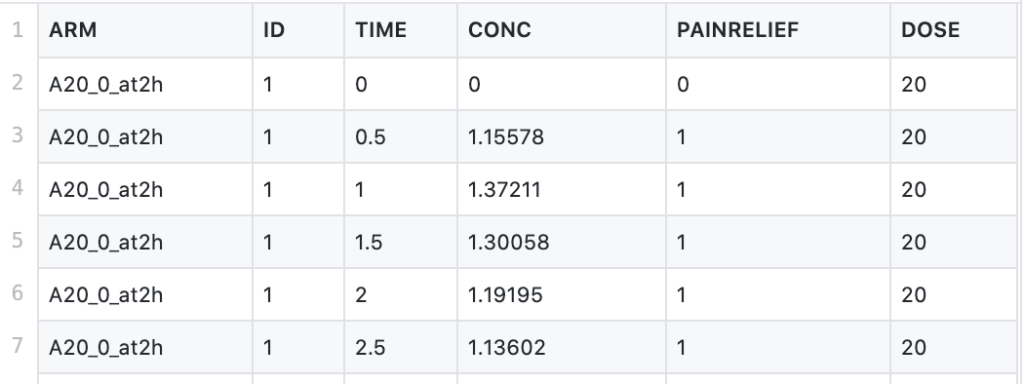
This CSV file contains data from a dose-ranging trial comparing placebo with three doses of a newly developed drug. The drug under investigation is an anti-inflammatory agent, and the study looks at self-reported pain relief and plasma concentration over time. The study features 4 arms (including the placebo arm), using doses of 5mg, 20mg, and 80mg, administered at time 0, and tracks the self-reported pain relief and drug concentration at 0, 0.5, 1, 1.5, 2, 2.5, and 3 to 8 hours.

The attributes of the dataset are as follows:

• ARM - arms of the clinical study
• TIME - time points of measured pain score and plasma concentration (in hrs)
• CONC - plasma concentration of the drug (in mg/L)
• PAINRELIEF - self-reported pain score (0=pain free, 1=mild pain, 2=moderate pain, 3=severe pain). A pain score over 2 is counted as "no relief"
• DOSE - the amount of drug administered (in mg)

Note that the maximum tolerated dose of the drug under investigation is 160 mg per day. Subjects are allowed to request re-medication if a reduction in pain is not felt within 2 hours after administration of the drug.

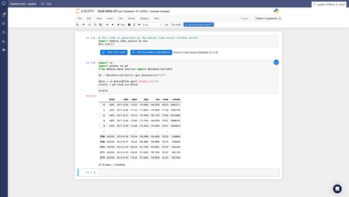
We load the data into a Julia DataFrame using the following.

pain_df = DataFrame(CSV.File("data/pk_painscore.csv"))

We can also check for missing values, although it appears that none are present.

colwise(x -> any(ismissing.(x)), pain_df)

Next, we can look at the different arms of the study that are included in the dataset.

unique(pain_df, "ARM")

The placebo arm is not relevant for the Non-Compartmental Analysis, so we can safely remove it.

pain_df = filter(row -> (row.ARM != "Placebo"), pain_df)

The NCA functions in Pumas require that the observations have an amount (AMT) and route (ROUTE) attributes. The route attribute indicates the route of administration. Possible choices are iv for intravenous, ev for extravascular, and inf for infusion. As the trial drug is not administered via an intravenous route, we'll add a ROUTE column to the data and set it to ev for all observations.

pain_df[:"ROUTE"] = "ev"

The requirement for the AMT attribute is that it should contain the relevant drug amount as a floating-point value at each dosing time, and otherwise should be set to missing. As each dose is administered at TIME=0 (the other entries are times of concentration and pain measurement), we create an AMT column as follows:

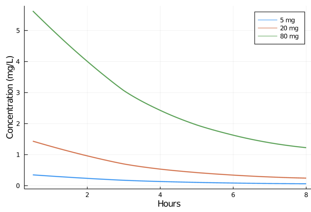
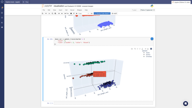
pain_df[:"AMT"] = ifelse.(pain_df.TIME .== 0, pain_df.DOSE, missing)

We can now visually inspect the change in plasma concentration over time in the 5, 20, and 80mg profiles:

Next, we call the Pumas read_nca function, which creates an NCAPopulation object containing preprocessed data for generation of all NCA values. See Parsing PumasNCADF for additional details.

pain_nca = read_nca(pain_df,
id = :ID,
time = :TIME,
conc = :CONC,
group = [:DOSE],
route = :ROUTE,
amt = :AMT)

We can now pass the preprocessed data to the Pumas NCAReport function, which calculates a wide range of relevant NCA metrics. The function returns a DataFrame so that we can look at its first ten rows.

nca_report = NCAReport(pain_nca, sigdig=2)

Note that the output above is column-wise truncated and shows only a handful of metrics. Let's see all the different properties calculated by NCAReport.

show(setdiff(names(nca_report), names(pain_df)))

"id", "doseamt", "tlag", "tmax", "cmax", "tlast", "clast", "clast_pred", "auclast", "kel", "half_life", "aucinf_obs", "aucinf_pred", "vz_f_obs", "cl_f_obs", "vz_f_pred", "cl_f_pred", "n_samples", "cmax_dn", "auclast_dn", "aucinf_dn_obs", "auc_extrap_obs", "aucinf_dn_pred", "auc_extrap_pred", "aumclast", "aumcinf_obs", "aumc_extrap_obs", "aumcinf_pred", "aumc_extrap_pred", "n_samples_kel", "rsq_kel", "rsq_adj_kel", "corr_kel", "intercept_kel", "kel_t_low", "kel_t_high", "span", "route", "run_status"

We can investigate specific metrics like maximum observed concentration (cmax) and extrapolated observed AUC (aucinf_obs). We can extract the two in a separate DataFrame.

cmax_auc_df = select(nca_report, [:DOSE, :cmax, :aucinf_obs])

We can group by study arm and calculate various statistics as mean and standard deviation.

gdf = groupby(cmax_auc_df, :DOSE);
combine(gdf, :aucinf_obs => mean, :aucinf_obs =>std, :cmax => mean, :cmax => std)

We can also plot the observed maximum concentration values and visually inspect the minimum, quartiles, median, and outliers by drug dose.

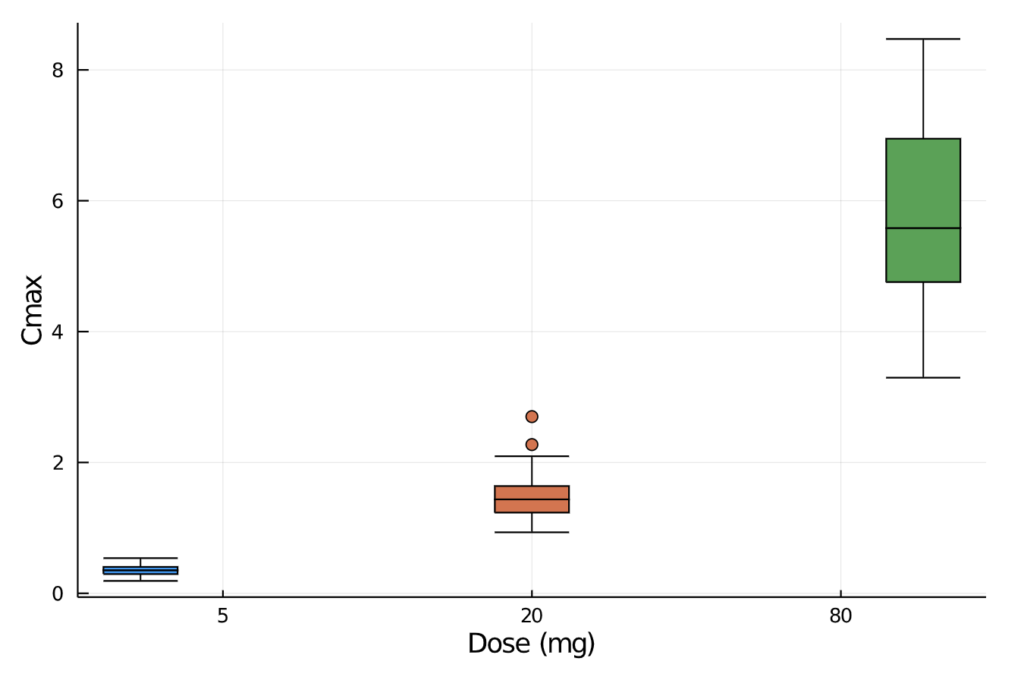
There are individual NCA functions that allow us to manually calculate the specific pharmacokinetic measurement of interest. For example:

• total clearance of the drug from plasma after oral administration (CL/F)
• terminal disposition rate constant (λz)
• mean residence time of the drug particles leaving the control volume (MRT)

and many others. We can merge all the metrics in a separate DataFrame for further analysis.

cl_f = NCA.cl(pain_nca)
lambda_z = NCA.lambdaz(pain_nca)
mrt = NCA.mrt(pain_nca)
metrics_df = innerjoin(cl_f, lambda_z, mrt, on=[:id, :DOSE], makeunique=true)

Based on our initial analysis and the monophasic morphology of the plasma concentration curves, it appears that one compartment model would fit the data. We can then proceed with pharmacokinetic modeling, testing the goodness of fit of various models. This example is further developed in the original Pumas tutorials here:

• A comprehensive introduction to Pumas - Part 1
• Non Compartmental Analysis

In this tutorial, we demonstrated how to carry out a simple Non-Compartmental Analysis. The openness of the Domino Enterprise MLOps platform allows us to use any language, tool, and framework while providing reproducibility, compute elasticity, knowledge discovery, and governance. Therefore, it is fairly easy to run Julia code and utilize third-party frameworks like Pumas AI.

References

[1] Gabrielsson J, Weiner D. Non-compartmental analysis. Methods Mol Biol. 2012;929:377-89. doi: 10.1007/978-1-62703-050-2_16. PMID: 23007438.
[2] Pumas AI Documentation, https://docs.pumas.ai
[3] Pumas AI website, https://pumas.ai/pumas