Genomic Ranges: An Introduction to Working with Genomic Data
Jack Fu2016-03-09 | 7 min read
Advancements in genome sequencing have outpaced even the high expectations that have placed upon them. We now have the capability to sequence a person’s entire genome for under $1000 - courtesy of Illumina’s HiSeq X Ten sequencer. In this post, I will introduce the workhorse package GenomicRanges that provides a convenient structure for representing genomic data and many built in functions for manipulating them.
Representing the Genome with a Coordinate System
The human genome is comprised of roughly 3 billion base pairs organized linearly on 23 pairs of chromosomes. Thus, an intuitive way to represent our genome is to use a coordinate system: “chromosome id” and “position along chromosome”. An annotation like chr1:129-131 would represent the 129th to the 131st base pair on chromosome 1.
Let us load GenomicRanges and create an example object to represent some genomic fragments:
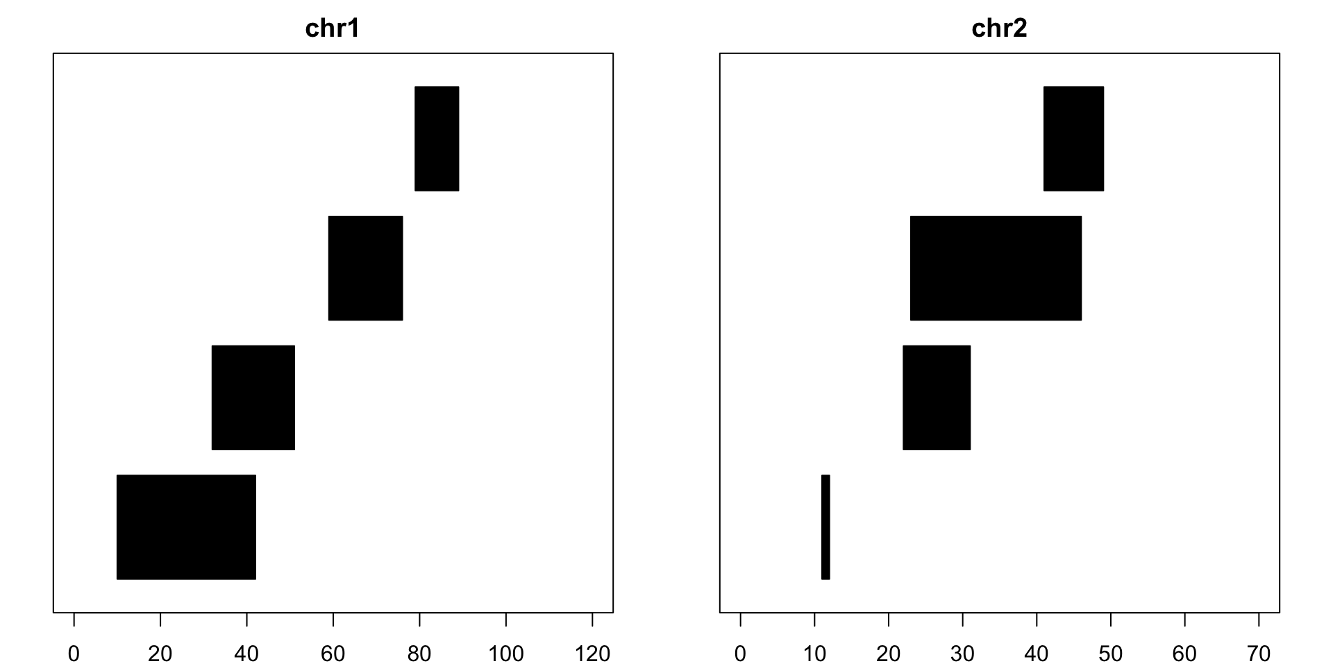
# Installationsource("https://bioconductor.org/biocLite.R") biocLite("GenomicRanges") The code below is how to create the an example GRanges object. The code entered here will create 8 segments on either chr1 or chr2, each with defined start and end points. Each read will also have strand information, indicating which direction the sequence is in. seglengths informs us the maximum length of chr1 and chr2.suppressMessages(library(GenomicRanges))example = GRanges(seqnames=c(rep("chr1", 4), rep("chr2", 4)), ranges = IRanges(start = c(10, 32, 59, 79, 11, 22, 23, 41), end=c(42, 51, 76, 89, 12, 31, 46, 49)), strand = rep(c("+", "-"), 4), seqlengths=c(chr1=120, chr2=70) )Now let’s take a look at R console representation of example:
example## GRanges object with 8 ranges and 0 metadata columns:## seqnames ranges strand## <Rle> <IRanges> <Rle>## [1] chr1 [10, 42] +## [2] chr1 [32, 51] -## [3] chr1 [59, 76] +## [4] chr1 [79, 89] -## [5] chr2 [11, 12] +## [6] chr2 [22, 31] -## [7] chr2 [23, 46] +## [8] chr2 [41, 49] -## -------## seqinfo: 2 sequences from an unspecified genomeand now let’s visualize what these pieces look like:
Assessors for GRanges Object
A GRanges object can be approached as an array and subset and modified as such:
example[1] ## GRanges object with 1 range and 0 metadata columns:## seqnames ranges strand## <Rle> <IRanges> <Rle>## [1] chr1 [10, 42] +## -------## seqinfo: 2 sequences from an unspecified genomeThe package also provides functions to access and modify information:
seqnames(example) ## factor-Rle of length 8 with 2 runs## Lengths: 4 4## Values : chr1 chr2## Levels(2): chr1 chr2width(example) ## [1] 33 20 18 11 2 10 24 9end(example) ## [1] 42 51 76 89 12 31 46 49start(example[1]) ## [1] 10start(example[1]) = 11 example ## GRanges object with 8 ranges and 0 metadata columns:## seqnames ranges strand## <Rle> <IRanges> <Rle>## [1] chr1 [11, 42] +## [2] chr1 [32, 51] -## [3] chr1 [59, 76] +## [4] chr1 [79, 89] -## [5] chr2 [11, 12] +## [6] chr2 [22, 31] -## [7] chr2 [23, 46] +## [8] chr2 [41, 49] -## -------## seqinfo: 2 sequences from an unspecified genomeOne could also store additional information for each piece to the GRanges object:
example$exon_id = 1:8 example ## GRanges object with 8 ranges and 1 metadata column:## seqnames ranges strand | exon_id## <Rle> <IRanges> <Rle> | <integer>## [1] chr1 [11, 42] + | 1## [2] chr1 [32, 51] - | 2## [3] chr1 [59, 76] + | 3## [4] chr1 [79, 89] - | 4## [5] chr2 [11, 12] + | 5## [6] chr2 [22, 31] - | 6## [7] chr2 [23, 46] + | 7## [8] chr2 [41, 49] - | 8## -------## seqinfo: 2 sequences from an unspecified genomeOperations of Individual Ranges
GenomicRanges also provide plenty of useful methods for carrying out “arithmetic” with the ranges:
Shift:
To move all pieces 10 base pair towards the end of the chromosomes one would do:
shift(example, 10) ## GRanges object with 8 ranges and 1 metadata column:## seqnames ranges strand | exon_id## <Rle> <IRanges> <Rle> | <integer>## [1] chr1 [21, 52] + | 1## [2] chr1 [42, 61] - | 2## [3] chr1 [69, 86] + | 3## [4] chr1 [89, 99] - | 4## [5] chr2 [21, 22] + | 5## [6] chr2 [32, 41] - | 6## [7] chr2 [33, 56] + | 7## [8] chr2 [51, 59] - | 8## -------## seqinfo: 2 sequences from an unspecified genomeTo move all pieces 5 base pairs toward the start of the chromosomes one would use:
shift(example, -5) ## GRanges object with 8 ranges and 1 metadata column:## seqnames ranges strand | exon_id## <Rle> <IRanges> <Rle> | <integer>## [1] chr1 [ 6, 37] + | 1## [2] chr1 [27, 46] - | 2## [3] chr1 [54, 71] + | 3## [4] chr1 [74, 84] - | 4## [5] chr2 [ 6, 7] + | 5## [6] chr2 [17, 26] - | 6## [7] chr2 [18, 41] + | 7## [8] chr2 [36, 44] - | 8## -------## seqinfo: 2 sequences from an unspecified genomeTo move each piece individually, one could use a vector:
shift(example, 1:8) ## GRanges object with 8 ranges and 1 metadata column:## seqnames ranges strand | exon_id## <Rle> <IRanges> <Rle> | <integer>## [1] chr1 [12, 43] + | 1## [2] chr1 [34, 53] - | 2## [3] chr1 [62, 79] + | 3## [4] chr1 [83, 93] - | 4## [5] chr2 [16, 17] + | 5## [6] chr2 [28, 37] - | 6## [7] chr2 [30, 53] + | 7## [8] chr2 [49, 57] - | 8## -------## seqinfo: 2 sequences from an unspecified genomeFlank
Flank is used to recover regions next to the input set. For a 3 base stretch upstream of example:
flank(example, 3) ## GRanges object with 8 ranges and 1 metadata column:## seqnames ranges strand | exon_id## <Rle> <IRanges> <Rle> | <integer>## [1] chr1 [ 8, 10] + | 1## [2] chr1 [52, 54] - | 2## [3] chr1 [56, 58] + | 3## [4] chr1 [90, 92] - | 4## [5] chr2 [ 8, 10] + | 5## [6] chr2 [32, 34] - | 6## [7] chr2 [20, 22] + | 7## [8] chr2 [50, 52] - | 8## -------## seqinfo: 2 sequences from an unspecified genomeEnter negative value for looking downstream, and the values can be a vector. Note that upstream and downstream is relative to the strand information of each piece.
Resize
The resize method resizes the pieces to the desired input length starting from the most upstream position relative to the direction of the strand:
resize(example, 10) ## GRanges object with 8 ranges and 1 metadata column:## seqnames ranges strand | exon_id## <Rle> <IRanges> <Rle> | <integer>## [1] chr1 [11, 20] + | 1## [2] chr1 [42, 51] - | 2## [3] chr1 [59, 68] + | 3## [4] chr1 [80, 89] - | 4## [5] chr2 [11, 20] + | 5## [6] chr2 [22, 31] - | 6## [7] chr2 [23, 32] + | 7## [8] chr2 [40, 49] - | 8## -------## seqinfo: 2 sequences from an unspecified genomeThere are numerous other methods that can be incredibly useful. See ?GRanges
Operations to a Set of Ranges
GenomicRanges also includes methods for aggregating the information of all the pieces in a particular GRanges instance. The following 3 methods are the most useful:
Disjoin
Disjoin reduces the ranges into the smallest set of unique, non-overlapping pieces that make up the original set. It is strand-specific by default, which means that the first and second piece are not considered to overlap unless told otherwise:
disjoin(example) ## GRanges object with 8 ranges and 0 metadata columns:## seqnames ranges strand## <Rle> <IRanges> <Rle>## [1] chr1 [11, 42] +## [2] chr1 [59, 76] +## [3] chr1 [32, 51] -## [4] chr1 [79, 89] -## [5] chr2 [11, 12] +## [6] chr2 [23, 46] +## [7] chr2 [22, 31] -## [8] chr2 [41, 49] -## -------## seqinfo: 2 sequences from an unspecified genomedisjoin(example, ignore.strand=T) ## GRanges object with 11 ranges and 0 metadata columns:## seqnames ranges strand## <Rle> <IRanges> <Rle>## [1] chr1 [11, 31] *## [2] chr1 [32, 42] *## [3] chr1 [43, 51] *## [4] chr1 [59, 76] *## [5] chr1 [79, 89] *## [6] chr2 [11, 12] *## [7] chr2 [22, 22] *## [8] chr2 [23, 31] *## [9] chr2 [32, 40] *## [10] chr2 [41, 46] *## [11] chr2 [47, 49] *## -------## seqinfo: 2 sequences from an unspecified genome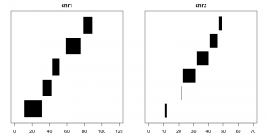
Reduce
Similarly, reduce creates the smallest merged set of unique, non-overlapping pieces that cover all the bases the original set does. Strand information is also taken into account by default and can be turned off:
reduce(example) ## GRanges object with 8 ranges and 0 metadata columns:## seqnames ranges strand## <Rle> <IRanges> <Rle>## [1] chr1 [11, 42] +## [2] chr1 [59, 76] +## [3] chr1 [32, 51] -## [4] chr1 [79, 89] -## [5] chr2 [11, 12] +## [6] chr2 [23, 46] +## [7] chr2 [22, 31] -## [8] chr2 [41, 49] -## -------## seqinfo: 2 sequences from an unspecified genomereduce(example, ignore.strand=T) ## GRanges object with 5 ranges and 0 metadata columns:## seqnames ranges strand## <Rle> <IRanges> <Rle>## [1] chr1 [11, 51] *## [2] chr1 [59, 76] *## [3] chr1 [79, 89] *## [4] chr2 [11, 12] *## [5] chr2 [22, 49] *## -------## seqinfo: 2 sequences from an unspecified genome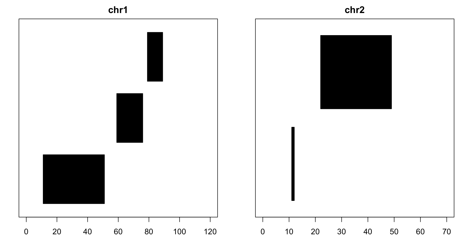
Coverage
If one needed to know how many times each base was covered by a read/piece, the coverage function is incredibly helpful:
coverage(example) ## RleList of length 2## $chr1## integer-Rle of length 120 with 9 runs## Lengths: 10 21 11 9 7 18 2 11 31## Values : 0 1 2 1 0 1 0 1 0## ## $chr2## integer-Rle of length 70 with 9 runs## Lengths: 10 2 9 1 9 9 6 3 21## Values : 0 1 0 1 2 1 2 1 0coverage(example)$chr1 ## integer-Rle of length 120 with 9 runs## Lengths: 10 21 11 9 7 18 2 11 31## Values : 0 1 2 1 0 1 0 1 0Operations Between Sets of Ranges
Finding Overlaps
GenomicRanges also provides a useful method for finding overlap between two sets of ranges. Let us suppose we are interested any of the pieces overlap our piece of interest target:
target = GRanges(seqnames="chr1", range=IRanges(start=5, 40)) ol = findOverlaps(target, example) ol ## Hits object with 2 hits and 0 metadata columns:## queryHits subjectHits## <integer> <integer>## [1] 1 1## [2] 1 2## -------## queryLength: 1## subjectLength: 8To see what piece(s) from example that overlaps target, we access the information stored in ol:
example[subjectHits(ol)] ## GRanges object with 2 ranges and 1 metadata column:## seqnames ranges strand | exon_id## <Rle> <IRanges> <Rle> | <integer>## [1] chr1 [11, 42] + | 1## [2] chr1 [32, 51] - | 2## -------## seqinfo: 2 sequences from an unspecified genomeTo see what piece(s) from example that overlaps target, we access the information stored in ol:
example[subjectHits(ol)] ## GRanges object with 2 ranges and 1 metadata column:## seqnames ranges strand | exon_id## <Rle> <IRanges> <Rle> | <integer>## [1] chr1 [11, 42] + | 1## [2] chr1 [32, 51] - | 2## -------## seqinfo: 2 sequences from an unspecified genomeApplied Example - Detecting Genomic Deletion
Now let us pull together everything that we have been looking at in this post to see if we can detect the presence of a deletion in some more realistically generated data.
With modern sequencing technology, the entire genome is not sequenced in one piece. DNA is usually prepped and shred into smaller fragments in a random process to allow for sequencing of the entire sequence. These smaller pieces are then fed into a machine that produces reads starting in random locations along those pieces. In the case of the most popular Illumina machines, the reads that are produced are 100 base pairs long. These reads are mapped back to the reference genome to find where they came from, and the location information can be loaded into R via GenomicRanges for evaluation.
If there is a deletion in the genome, one would expect to find no reads coming from a certain area. Let us take a look at the GRanges object containing the location information for 2000 simulated reads from an individual. This resembles what might be stored in a GRanges object after sequencing a fictitious chromosome Z that is 1000 base pair long in the reference:
set.seed(1337) # Ensure reproducibility starts = floor(runif(2000)*900)+1 reads = GRanges(seqname="chrZ", ranges=IRanges(start=starts, end=starts+99)) reads ## GRanges object with 2000 ranges and 0 metadata columns:## seqnames ranges strand## <Rle> <IRanges> <Rle>## [1] chrZ [519, 618] *## [2] chrZ [509, 608] *## [3] chrZ [ 67, 166] *## [4] chrZ [409, 508] *## [5] chrZ [336, 435] *## ... ... ... ...## [1996] chrZ [181, 280] *## [1997] chrZ [224, 323] *## [1998] chrZ [499, 598] *## [1999] chrZ [ 63, 162] *## [2000] chrZ [ 15, 114] *## -------## seqinfo: 1 sequence from an unspecified genome; no seqlengthsWe can use reduce to see what parts of chrZ is covered by reads:
reduce(reads) ## GRanges object with 1 range and 0 metadata columns:## seqnames ranges strand## <Rle> <IRanges> <Rle>## [1] chrZ [1, 999] *## -------## seqinfo: 1 sequence from an unspecified genome; no seqlengthsLet us also take a look at the coverage of each base from this set of reads
plot(coverage(reads)$chrZ, ty="l", main="Coverage of Reads of ChrZ", xlab="Coordinates along ChrZ", ylab="Coverage") 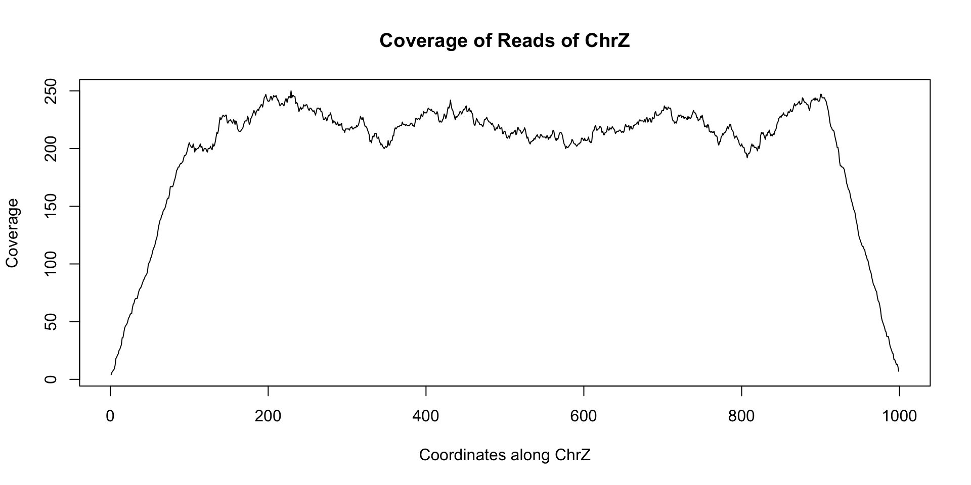
Note the relatively stable coverage along the length of chrZ. This appears to indicate that there is no deletion along chrZ. Now let us look at another dataset reads_2 that came from a separate individual:
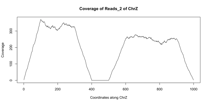
starts = c(floor(runif(1000)*300), floor(runif(1000)*400)+500)+1 reads_2 = GRanges(seqname="chrZ", ranges=IRanges(start=starts, end = starts+99)) reduce(reads_2) ## GRanges object with 2 ranges and 0 metadata columns:## seqnames ranges strand## <Rle> <IRanges> <Rle>## [1] chrZ [ 1, 399] *## [2] chrZ [501, 999] *## -------## seqinfo: 1 sequence from an unspecified genome; no seqlengthsplot(coverage(reads_2)$chrZ, ty="l", main="Coverage of Reads_2 of ChrZ", xlab="Coordinates along ChrZ", ylab="Coverage") 
Note the area of low to no coverage in the plot and the gap in sequence from reduce - this seems to indicate that a segment of chrZ is deleted in the second subject between bases 400 and 500. Now we wish to find if this deletion overlaps any annotated regions in the reference genome. This can be achieved using findOverlaps and a GRanges object containing the annotation information. There are many such annotations that have been created that can be loaded into R. For our example we can use the following annotation GRanges object annotation:
annotation ## GRanges object with 4 ranges and 1 metadata column:## seqnames ranges strand | Gene_id## <Rle> <IRanges> <Rle> | <character>## [1] chrZ [100, 150] * | Gene_1## [2] chrZ [200, 250] * | Gene_2## [3] chrZ [400, 550] * | Gene_3## [4] chrZ [700, 750] * | Gene_4## -------## seqinfo: 1 sequence from an unspecified genome; no seqlengthsol = findOverlaps(GRanges(seqnames="chrZ", ranges=IRanges(start=500, end=600)), annotation) annotation[subjectHits(ol)] ## GRanges object with 1 range and 1 metadata column:## seqnames ranges strand | Gene_id## <Rle> <IRanges> <Rle> | <character>## [1] chrZ [400, 550] * | Gene_3## -------## seqinfo: 1 sequence from an unspecified genome; no seqlengthsThus, it would appear that Gene_3 is deleted in the second subject - this information can be passed on to downstream lab scientists for verification as well as general cataloging.
Congratulations on learning the basics of dealing with genomic read data in R using GenomicRanges. In future posts, I will go over in more detail some the technical artifacts of sequencing that have been reported and require adjustment. For instance, the reads that are generated from the genome do not come so uniformly along the entire genome. Furthermore, we will look at some more advanced methods to detect mutations in genetic read data.

Jack Fu is a Postdoctoral Research Fellow at Harvard Medical School. Previously, he was a PhD student in the Biostatistics Department at the Johns Hopkins Bloomberg School of Public Health, where he worked on projects involving genomic data.
RELATED TAGS
SHARE
Other posts you might be interested in


Subscribe to the Domino Newsletter
Receive data science tips and tutorials from leading Data Science leaders, right to your inbox.
By submitting this form you agree to receive communications from Domino related to products and services in accordance with Domino's privacy policy and may opt-out at anytime.