Accelerating model velocity through Snowflake Java UDF integration
Nikolay Manchev2021-06-15 | 15 min read
Over the next decade, the companies that will beat competitors will be “model-driven” businesses. These companies often undertake large data science efforts in order to shift from “data-driven” to "model-driven" operations, and to provide model-underpinned insights to the business.
The typical data science journey for a company starts with a small team that is tasked with a handful of specific problems. Tracking and managing a small number of experiments that deal with data in Excel is fairly straightforward. The challenges surface once the company hits the scalability wall. At a certain point, as the demand keeps growing, the data volumes rapidly increase. Data is no longer stored in CSV files, but in a dedicated, purpose built data lake / data warehouse. Individual laptops are no longer capable of processing the required volumes. The data science team grows and people can't work in isolation anymore - they need to be able to share knowledge, handover projects, and have validation and reproducibility capabilities at their disposal.
To properly scale data science, companies need a holistic system to develop, deploy, monitor, and manage models at scale – a system of record for their data science. This is the core functionality of the Domino’s Enterprise MLOps platform - a system that enables fast, reproducible, and collaborative work on data products like models, dashboards, and data pipelines. Similarly, Snowflake's Data Cloud has been gaining momentum and is now one of the key players in cloud-based data storage and analytics (the data warehouse-as-a-service space).
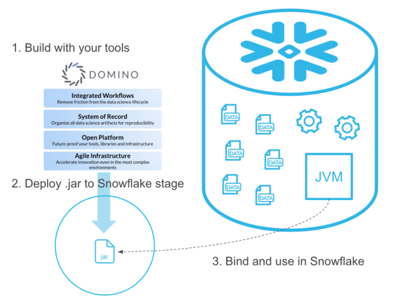
Both platforms are cloud agnostic so they can run in Azure, GCP, and AWS. Joint customers already use Domino data connectors to retrieve and write data between the Domino environment and the Snowflake Data Cloud. The recently announced partnership between Domino Data Lab and Snowflake enhanced this experience with the integration of Snowflake’s Snowpark and Java UDFs in Domino. Snowpark is a new developer experience, which enables data scientists to leverage their favourite tools and deploy code directly within Snowflake.
In this blog post we'll focus on the UDF capabilities provided by the two platforms.
Why Snowflake UDFs
Generally speaking, a User Defined Function (UDF), in the context of relational databases, is a mechanism for extending the functionality of the underlying database. Moreover, such a function can be evaluated within standard SQL queries, but it can be written in a language different to SQL. This definition makes UDFs somewhat similar to stored procedures, but there are a number of key differences between the two. Snowflake stored procedures use JavaScript and, in most cases, SQL. UDFs do support JavaScript and SQL, but they can also be written in other languages like Java and Scala. Stored procedures are invoked directly (via a CALL command), but UDFs are called as part of a statement. Therefore, if we need a value that can be used within the statement or if we need to produce a value for every input row, our best bet is UDFs.
Most importantly, UDFs are executed directly in Snowflake. If Big Data has taught us anything, it is that with large volumes and high velocity data, it is advisable to move the computation to where the data resides. Shifting gigabytes and even terabytes of data between instances (or even different cloud providers) can have substantial impact on performance, and negatively impact the Data Science team's capability to maintain high model velocity and to support the innovation efforts within the company. This is where UDFs come into play and they could be a versatile mechanism that improves the performance and streamlines a number of use cases.
For example:
- Accelerated model building and scoring
- A model training Java UDF can be loaded in Snowflake, and the model can be automatically rebuilt as new data comes in, without the need to transfer data between instances.
- A pre-trained model can be loaded as an UDF in Snowflake for the purposes of scoring incoming data as soon as it lands into the database (e.g. anomaly detection).
- Advanced data wrangling and preprocessing pipelines
- A Java UDF can use a wider range of techniques for data cleansing, feature engineering, and mode advanced preprocessing, compared to what is available in SQL.
- Existing preprocessing, data ingestion, and data quality processes can be converted from Java/Spark into Java UDFs. These pipelines can then run natively in Snowflake with their execution and reproducibility managed by Domino.
- Enhanced Business Intelligence capabilities
- UDFs that do complex processing, aggregation, and transformation can be leveraged by Business Intelligence tools via SQL calls. This enables BI products running in Domino (e.g. Apache SuperSet) to extract and apply advanced calculations and aggregations, which are normally not available in the tool or plain SQL.
Connecting to Snowflake from Domino
Connecting the Snowflake from Domino is trivial, as the Snowflake libraries and Snowflake drivers are already included in the default Domino Analytics Distribution compute environment. We also covered the process of setting up credentials and creating the initial connection in a previous blog post.
After connecting to Snowflake, we run a simple SELECT statement to confirm that our connection works properly and to verify the Snowflake version.
import os
import snowflake.connector as sf
ctx = sf.connect(
    user=os.environ["SNOWFLAKE_USER"],
    password=os.environ["SNOWFLAKE_PASSWORD"],
    account=os.environ["SNOWFLAKE_ACCOUNT"])
cur = ctx.cursor()
cur.execute("SELECT current_version()")
cur.fetchone()[0]'5.21.2'For the purposes of this demo, we created a table in Snowflake using the following DDL:
CREATE OR REPLACE TABLE DOMINO_DEMONSTRATIONS.PUBLIC.AUTOMPG (
	MPG NUMBER(38,0),
	CYLINDERS NUMBER(38,0),
	DISPLACEMENT NUMBER(38,0),
	HORSEPOWER NUMBER(38,0),
	WEIGHT NUMBER(38,0),
	ACCELERATION FLOAT,
	YEAR NUMBER(38,0),
	ORIGIN NUMBER(38,0),
	NAME VARCHAR(16777216)
);
The table is populated with the AutoMPG dataset, which can be downloaded from Kaggle. We can run a simple SELECT and fetch the first 3 rows from the AUTOMPG table.
cur.execute("USE DATABASE DOMINO_DEMONSTRATIONS")
res = cur.execute("SELECT * FROM AUTOMPG LIMIT 3")
for row in res:
    print(row)
(18, 8, 307, 130, 3504, 12.0, 70, 1, 'chevrolet chevelle malibu')
(15, 8, 350, 165, 3693, 11.5, 70, 1, 'buick skylark 320')
(18, 8, 318, 150, 3436, 11.0, 70, 1, 'plymouth satellite')Now that connectivity has been confirmed, we can move to UDFs.
Using Snowflake Java UDFs from Domino
We start by defining a simple Java UDF. Our first function is a very basic Java method that simply returns the sum of two numbers. The Java code looks like this:
public static int add(int x, int y) {
    return x + y;
}
This static method accepts two arguments x and y, and returns their sum. Generally, Snowflake supports two types of UDFs:
- pre-compiled UDF, which are imported as JAR files and can contain multiple Java functions
- in-line UDF, which normally contain a single function and are compiled on the fly by Snowflake
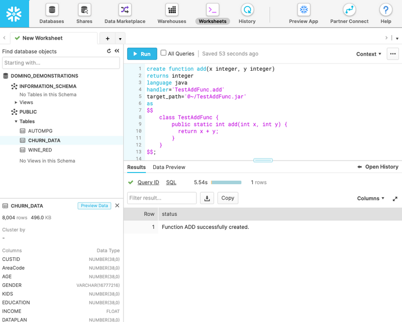
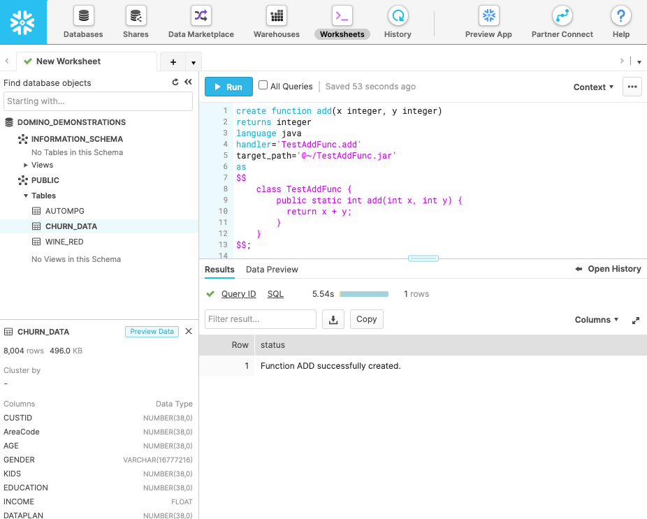
In this example we will use an in-line UDF, so all we need to do is to wrap the Java code in a CREATE FUNCTION statement.
create function add(x integer, y integer)
returns integer
language java
handler='TestAddFunc.add'
target_path='@~/TestAddFunc.jar'
as
$$
    class TestAddFunc {
        public static int add(int x, int y) {
          return x + y;
        }
    }
$$;
The syntax above is fairly self explanatory - the Java code is wrapped by a pair of $ signs. The target_path clause tells Snowflake what file name to use for the compiled Java code, and the handler clause gives the name of the Java method that needs to be executed when the UDF is called. Running this DDL in Snowflake results in a "Function ADD successfully completed" message.
We can now test the function from our Domino Workspace (JupyterLab in this case):
cur.execute("SELECT ADD(5,2)")
cur.fetchone()[0]7Let's define another function. This one will use the formula 235.215/(1 US mpg) = 235.215 L/100 km, to convert MPGs to liters per 100km. The DDL for the function looks like this:
create function l100km(mpg float)
returns double
language java
handler='L100KMFunc.l100km'
target_path='@~/L100KMAddFunc.jar'
as
$$
    class L100KMFunc {
        public static double l100km(float mpg) {
          return (235.214583 / mpg);
        }
    }
$$;
We can call this function with the MPG column from our AUTOMPG table, to get the TOP 5 most fuel efficient vehicles in the dataset, simultaneously converting the MPG into L/100km.
res = cur.execute("SELECT NAME, ROUND(L100KM(MPG),2) AS \"L/100KM\" FROM AUTOMPG ORDER BY \"L/100KM\" LIMIT 5")
for row in res:
    print(row)
('mazda glc', 5.0)
('honda civic 1500 gl', 5.23)
('vw rabbit c (diesel)', 5.35)
('vw pickup', 5.35)
('vw dasher (diesel)', 5.47)The result set confirms that the function is called on a row by row basis, and the MPG to L/100km conversion is performed on the fly. This is a fairly simple example, as you can certainly do this calculation in pure SQL, but the key point here is that using this approach you can unleash the full power of Java and perform sophisticated manipulations on the fly.
Now let's implement a simple machine learning scoring function against our test data. Recall that Domino enables teams to use different tools and languages, so to make this example slightly more exciting, suppose one of our colleagues used R to fit a linear model against the AutoMPG data. The model explains the relationship between MPG and HORSEPOWER, and the R code that produces it looks like this:
> head(autompg)
  mpg cylinders displacement horsepower weight acceleration model.year origin                  car.name
1  18         8          307        130   3504         12.0         70      1 chevrolet chevelle malibu
2  15         8          350        165   3693         11.5         70      1         buick skylark 320
3  18         8          318        150   3436         11.0         70      1        plymouth satellite
4  16         8          304        150   3433         12.0         70      1             amc rebel sst
5  17         8          302        140   3449         10.5         70      1               ford torino
6  15         8          429        198   4341         10.0         70      1          ford galaxie 500
> model <- lm(formula=mpg~horsepower, data=autompg)> summary(model)Call:
lm(formula = mpg ~ horsepower, data = autompg)Residuals:Min 1Q Median 3Q Max-13.5710 -3.2592 -0.3435 2.7630 16.9240Coefficients:Estimate Std. Error t value Pr(>|t|)(Intercept) 39.935861 0.717499 55.66 <2e-16 ***horsepower -0.157845 0.006446 -24.49 <2e-16 ***---Signif. codes: 0 ‘***’ 0.001 ‘**’ 0.01 ‘*’ 0.05 ‘.’ 0.1 ‘ ’ 1Residual standard error: 4.906 on 390 degrees of freedom(6 observations deleted due to missingness)Multiple R-squared: 0.6059, Adjusted R-squared: 0.6049F-statistic: 599.7 on 1 and 390 DF, p-value: < 2.2e-16Using the intercept and the horsepower coefficient, we can define the following UDF function:
create function mpgPredict(mpg float)
returns double
language java
handler='ML.mpgPredict'
target_path='@~/ML3.jar'
as
$$
    class ML {
        public static double mpgPredict(float horsepower) {
          float intercept = 39.935861f;
          float hp_coeff =  -0.157845f;
          return intercept + hp_coeff * horsepower;
        }
    }
$$;
Note, that we have hard-coded the coefficients for simplicity, but we could as easily pull them from an external file or another table, which gets updated after each model retraining. Once the predictive function is in place, we can use it to see how well the predictions match the existing data.
res = cur.execute("SELECT NAME, ROUND(MPGPREDICT(HORSEPOWER),2), MPG FROM AUTOMPG LIMIT 5")
for row in res:
    print(row)
('chevrolet chevelle malibu', 19.42, 18)
('buick skylark 320', 13.89, 15)
('plymouth satellite', 16.26, 18)
('amc rebel sst', 16.26, 16)
('ford torino', 17.84, 17)We can also use the UDF to score unseen data. For example, we can calculate the expected MPG for a Toyota RAV4 - a vehicle, which is not in the original AutoMPG database.
cur.execute("SELECT 'TOYOTA RAV4' AS MODEL, ROUND(MPGPREDICT(163),2) AS MPG");
cur.fetchone()
('TOYOTA RAV4', 14.21)Pre-compiled UDFs
A Java UDF is stored in a JAR file. Snowflake automatically handles the compilation and packaging of in-line UDFs. Pre-compiled UDFs, however, require some extra upfront work.
The organisation of the JAR file follows the standard Java Archive convention. If you are not familiar with the standard JAR file structure, you can read the Packaging Programs in JAR Files tutorial in the official Java documentation.
At a very high level, the steps you need to go through to create your own pre-compiled UDF are as follows:
- Write the Java class(es), which contains the function(s) that you are planning to expose as UDF.
- Use a Java compiler (javac) to compile the source code to .class files.
- Package your .class file(s) into a JAR file. You can use the Java jar command.
- Add a manifest file, which contains meta information about what exactly is included in your JAR file.
After the JAR file is ready, it needs to be copied to an external or named internal stage in Snowflake, which must be readable by the owner of the UDF. The recommended way to do this is to use a PUT command, for example:
put
    file:///absolute_path_to_the_jar_file/jar_file_name.jar
    @~/udf_stage_dir/
    auto_compress = false
    overwrite = true
    ;
Note the overwrite flag above. This option is helpful when the JAR file is part of some CI/CD pipeline (e.g. we are retraining a model and packaging it into a JAR file on a schedule), and it needs to be replaced regularly. If this is the case, Snowflake recommends doing the UDF update when no calls to the function can be made.
The Java Archive format supports a wide range of functionality, including electronic signing, compression, version control, version consistency enforcement (package sealing) and others. This brings extra benefits like security, versioning, and portability, but more importantly, archives allow you to package additional files alongside your classes. These can be pre-trained models, vector space models, additional Java classes (e.g. custom machine learning algorithms), etc.
Summary
In this blog post we covered some of the key advantages of the Domino - Snowflake UDF integration. The Domino Data Science platform can interface with UDFs in Snowflake and enable data scientists to use them as building blocks in complex pipelines (for example for data preprocessing and data wrangling), or for training models and scoring data. Key advantages of this approach are that it enables access to complex features from languages like Scala and Java, and it eliminates the need to move data between instances and clouds.
Although in this article we focused on one-way use-cases (i.e. calling UDFs from Domino), a bi-directional communication is also fully supported. One can envision a UDF in Snowflake that makes calls to Model APIs or Domino Model Manager, to score incoming data on the fly, or to perform on-line checks for data drift as soon as new samples hit the database.
This type of automation enables models to respond quicker, removes scalability issues caused by large data volumes or insufficient compute resources, makes data science teams more productive, and reduces the cost of training and running models at scale.
Moreover, as all the code for accessing and creating UDFs can reside in Domino, the platform transparently provides versioning, traceability, and reproducibility for all the deliverables created by the Data Science team. This facilitates knowledge discovery, handover, and regulatory compliance, and allows the individual data scientists to focus on work that accelerates research and speeds model deployment.
About Domino
Domino’s Enterprise MLOps platform addresses the problems that make it hard to scale data science by:
- Supporting the broadest ecosystem of open-source and commercial tools and infrastructure.
- Providing repeatability, and reproducibility across the end-to-end lifecycle of every experiment, no matter what tool has been used in the development process.
- Accelerating the full, end-to-end lifecycle from ideation to production by providing consistent, streamlined experience in a single platform.
- Satisfying IT requirements for security, governance, compliance, and collaboration.
The holistic approach outlined above is a key characteristic that makes Domino the Enterprise MLOps platform trusted by over 20% of the Fortune 100 companies.
About Snowflake
Snowflake delivers the Data Cloud—a global network where thousands of organizations mobilize data with near-unlimited scale, concurrency, and performance. Some of the key features provided by the Snowflake's Data Cloud platform include:
- A true SaaS offering with virtually unlimited scalability via elastic virtual compute instances and virtual storage services.
- Support for a wide range of programming languages like Go, Java, .NET, Python, C, Node.js, including ANSI SQL compatibility.
- Support for a variety of data structures (e.g. CSVs, XML, JSON, Parquet and others).
- Straightforward connectivity via ODBC, JDBC, native connectors (e.g. Python, Spark), third-party ETL & BI tools integration (e.g. Informatica, ThoughtSpot and others)
- A fully managed service with near-zero maintenance.

Nikolay Manchev is the Principal Data Scientist for EMEA at Domino Data Lab. In this role, Nikolay helps clients from a wide range of industries tackle challenging machine learning use-cases and successfully integrate predictive analytics in their domain specific workflows. He holds an MSc in Software Technologies, an MSc in Data Science, and is currently undertaking postgraduate research at King's College London. His area of expertise is Machine Learning and Data Science, and his research interests are in neural networks and computational neurobiology.
Subscribe to the Domino Newsletter
Receive data science tips and tutorials from leading Data Science leaders, right to your inbox.
By submitting this form you agree to receive communications from Domino related to products and services in accordance with Domino's privacy policy and may opt-out at anytime.