SHAP and LIME Python Libraries: Part 1 - Great Explainers, with Pros and Cons to Both
Josh Poduska2018-12-05 | 6 min read
This blog post provides a brief technical introduction to the SHAP and LIME Python libraries, followed by code and output to highlight a few pros and cons of each. If interested in a visual walk-through of this post, consider attending the webinar.
Introduction
Model explainability is a priority in today's data science community. As data scientists, we want to prevent model bias and help decision makers understand how to use our models in the right way. Data science leaders and executives are mindful of existing and upcoming legislation that requires models to provide evidence of how they work and how they avoid mistakes (e.g., SR 11-7 and The FUTURE of AI Act).
Part 1 in this blog post provides a brief technical introduction to the SHAP and LIME Python libraries, followed by code and output to highlight a few pros and cons of each. Part 2 will explore these libraries in more detail by applying them to a variety of Python models. The goal of these posts is to familiarize readers with how to use these libraries in practice and how to interpret their output, helping you leverage model explanations in your own work.
SHAP vs. LIME
SHAP and LIME are both popular Python libraries for model explainability. SHAP (SHapley Additive exPlanation) leverages the idea of Shapley values for model feature influence scoring. The technical definition of a Shapley value is the “average marginal contribution of a feature value over all possible coalitions.” In other words, Shapley values consider all possible predictions for an instance using all possible combinations of inputs. Because of this exhaustive approach, SHAP can guarantee properties like consistency and local accuracy. LIME (Local Interpretable Model-agnostic Explanations) builds sparse linear models around each prediction to explain how the black box model works in that local vicinity. In their NIPS paper, the authors of SHAP show that Shapley values provide the only guarantee of accuracy and consistency and that LIME is actually a subset of SHAP but lacks the same properties. For further study, I found the GitHub sites SHAP GitHub and LIME GitHub helpful resources:
So why would anyone ever use LIME? Simply put, LIME is fast, while Shapley values take a long time to compute. For you statisticians out there, this situation reminds me somewhat of Fisher’s Exact Test versus a Chi-Squared Test on contingency tables. Fisher’s Exact Test provides the highest accuracy possible because it considers all possible outcomes, but it takes forever to run on large tables. This makes the Chi-Squared Test, a distribution-based approximation, a nice alternative.
The SHAP Python library helps with this compute problem by using approximations and optimizations to greatly speed things up while seeking to keep the nice Shapley properties. When you use a model with a SHAP optimization, things run very fast and the output is accurate and reliable. Unfortunately, SHAP is not optimized for all model types yet.
For example, SHAP has a tree explainer that runs fast on trees, such as gradient boosted trees from XGBoost and scikit-learn and random forests from sci-kit learn, but for a model like k-nearest neighbor, even on a very small dataset, it is prohibitively slow. Part 2 of this post will review a complete list of SHAP explainers. The code and comments below document this deficiency of the SHAP library on the Boston Housing dataset.
# Load Libraries
import pandas as pd
import sklearn
from sklearn.model_selection import train_test_split
import sklearn.ensemble
import numpy as np
import lime
import lime.lime_tabular
import shap
import xgboost as xgb
import matplotlib
import matplotlib.pyplot as plt
from mpl_toolkits.mplot3d import axes3d, Axes3D
import seaborn as sns
import time
%matplotlib inline
# Load Boston Housing Data
X,y = shap.datasets.boston()
X_train,X_test,y_train,y_test = train_test_split(X, y, test_size=0.2, random_state=0)
X,y = shap.datasets.boston()
X_train,X_test,y_train,y_test = train_test_split(X, y, test_size=0.2, random_state=0)
# K Nearest Neighbor
knn = sklearn.neighbors.KNeighborsRegressor()
knn.fit(X_train, y_train)
# Create the SHAP Explainers
# SHAP has the following explainers: deep, gradient, kernel, linear, tree, sampling
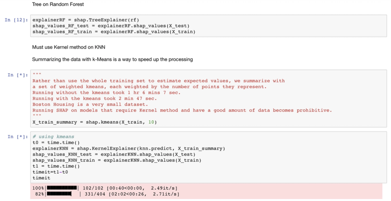
# Must use Kernel method on knn
# Summarizing the data with k-Means is a trick to speed up the processing
"""Rather than use the whole training set to estimate expected values, we summarize with a set of weighted kmeans,each weighted by the number of points they represent. Running without kmeans took 1 hr 6 mins 7 sec.Running with kmeans took 2 min 47 sec. Boston Housing is a small dataset.Running SHAP on models that require the Kernel method becomes prohibitive."""
# build the kmeans summary
X_train_summary = shap.kmeans(X_train, 10)
# using the kmeans summary
t0 = time.time()
explainerKNN = shap.KernelExplainer(knn.predict,X_train_summary)
shap_values_KNN_test = explainerKNN.shap_values(X_test)
t1 = time.time()
timeit=t1-t0timeit
# without kmeans a test run took 3967.6232330799103 seconds
"""t0 = time.time() explainerKNN = shap.KernelExplainer(knn.predict, X_train) shap_values_KNN_test = explainerKNN.shap_values(X_test) t1 = time.time() timeit=t1-t0 timeit"""
# now we can plot the SHAP explainer
shap.force_plot(explainerKNN.expected_value, shap_values_KNN_test[j], X_test.iloc[[j]])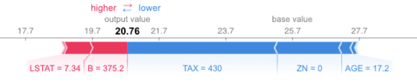
Running SHAP on a knn model built on the Boston Housing dataset took over an hour, which is a tough pill to swallow. We can get that down to three minutes if we sacrifice some accuracy and reliability by summarizing the data first with a k-means algorithm. As an alternative approach, we could use LIME. LIME runs instantaneously with the same knn model and does not require summarizing with k-means. See the code and output below. Note that LIME’s output is different than the SHAP output, especially for features AGE and B. With LIME not having the same accuracy and consistency properties as Shapley Values, and with SHAP using a k-means summary before calculating influence scores, it's tough to tell which comes closer to the correct answer.
exp = explainer.explain_instance(X_test.values[j], knn.predict, num_features=5)
exp.show_in_notebook(show_table=True)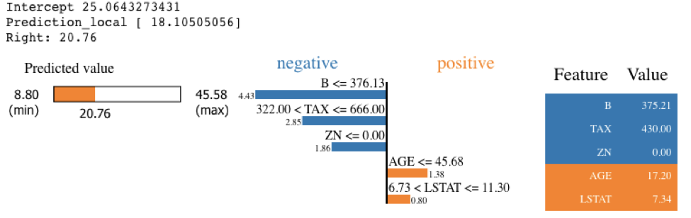
While LIME provided a nice alternative in the knn model example, LIME is unfortunately not always able to save the day. It doesn’t work out-of-the-box on all models. For example, LIME cannot handle the requirement of XGBoost to use xgb.DMatrix() on the input data. See below for one attempt to call LIME with the XGBoost model. There are potential hacks that could get LIME to work on this model, including creating your own prediction function, but the point is LIME doesn’t automatically work with the XGBoost library.
xgb_model = xgb.train({"objective":"reg:linear"}, xgb.DMatrix(X_train, label=y_train))
    max_features="auto", max_leaf_nodes=None,
    min_impurity_decrease=0.0, min_impurity_split=None,
    min_samples_leaf=1, min_samples_split=2,
    min_weight_fraction_leaf=0.0, n_estimators=10, n_jobs=1, oob_score=False,
    random_state=None, verbose=0, warm_start=False)

# LIME has one explainer for all models
explainer = lime.lime_tabular.LimeTabularExplainer(X_train.values,
    feature_names=X_train.columns.values.tolist(),
    class_names=["price"],
    categorical_features=categorical_features,
    verbose=True,
    mode="regression")

# Out-of-the-box LIME cannot handle the requirement of XGBoost to use xgb.DMatrix() on the input data
xgb_model.predict(xgb.DMatrix(X_test.iloc[[j]]))
expXGB = explainer.explain_instance(X_test.values[j], xgb_model.predict, num_features=5)
expXGB.show_in_notebook(show_table=True)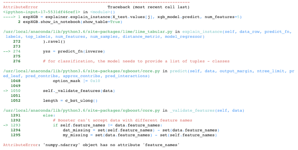
On the other hand, SHAP is optimized for XGBoost and provides fast, reliable results. The following code runs very fast. It uses the TreeExplainer from the SHAP library, which is optimized to trace through the XGBoost tree to find the Shapley value estimates.
explainerXGB = shap.TreeExplainer(xgb_model)
shap_values_XGB_test = explainerXGB.shap_values(X_test)
shap.force_plot(explainerXGB.expected_value, shap_values_XGB_test[j], X_test.iloc[[j]])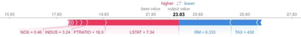
Conclusion
Hopefully, this post has given you a few pointers on how to choose between SHAP and LIME and brought to light some of the limitations of each. While both approaches have their strengths and limitations, I personally prefer to use SHAP when I can and rely on LIME when SHAP’s compute costs are too high. Stay tuned for my next post on this topic, which will provide multiple examples of how to use these libraries on a variety of models and also show how to interpret their output.

Josh Poduska is the Chief Field Data Scientist at Domino Data Lab and has 20+ years of experience in analytics. Josh has built data science solutions across domains including manufacturing, public sector, and retail. Josh has also managed teams and led data science strategy at multiple companies, and he currently manages Domino’s Field Data Science team. Josh has a Masters in Applied Statistics from Cornell University. You can connect with Josh at https://www.linkedin.com/in/joshpoduska/
RELATED TAGS
SHARE

Subscribe to the Domino Newsletter
Receive data science tips and tutorials from leading Data Science leaders, right to your inbox.
By submitting this form you agree to receive communications from Domino related to products and services in accordance with Domino's privacy policy and may opt-out at anytime.